Sampling the Solid Angle of Area Light Sources
April 8, 2018
$\newcommand{\c}{\textbf{c}}$ $\newcommand{\x}{\textbf{x}}$ $\newcommand{\r}{\textit{r}}$ $\newcommand{\w}{\hat{\omega}}$ $\newcommand{\a}{\hat{\textit{a}}}$ $\newcommand{\n}{\hat{\textit{n}}}$ $\newcommand{\v}{\hat{\textit{v}}}$ $\newcommand{\d}{\hat{\textit{d}}}$ $\newcommand{\u}{\hat{\textit{u}}}$ $\newcommand{\thetamax}{\theta_{max}}$
With ray tracing mania taking over thanks to the announcement of DXR now seems like a great time for me to write about the next subject I wanted to write about: sampling the solid angle of area lights. While the concept was described in research at least two decades ago I’ve found that most books and blog posts that mention sampling area lights tend to describe sampling the surface area of the light source. I’ll start with an explanation of why you would want to sample the solid angle of an area light as well as mention the cons of doing so. I’ll then dig into the gritty details of how to sample a spherical area light. Finally, I’ll leave you with some references for sampling the solid angle of other area light shapes.
To give you some intuition for why we would want to sample the solid angle of an area light I’ll start with this exceptional piece of programmer art:
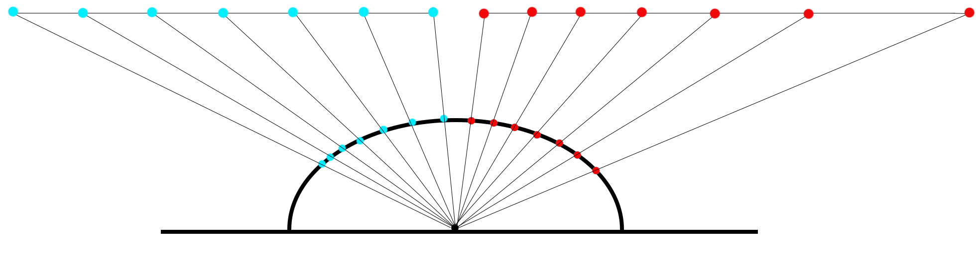
If it’s not clear, this is a 2D view of two rectangular area lights. On the left, the blue samples are distributed evenly over the area of the light and, on the right, the red samples are distributed evenly over the solid angle of the light. On the left side you can see that the samples are somewhat sparse near the top of the hemisphere and get more dense near the horizon. If that light source were to extend even further to the left you can imagine how the samples would become incredibly dense at the horizon. There are two factors here that contibute to this being a poor sample density. Any sample taken will have its lighting attentuated by the cosine term, which is lowest near the horizon, as well as by the recriprical of the square of the distance, which is also going to be the lowest near the horizon. Both of those factors mean that sampling of the area of the light source is prone to sampling the most where it contributes the least in this example. However, on the right side the samples are more dense where the cosine term is greatest and where the distance is shortest.
There’s another distrubtion we could sample that would give us even better results. Here’s a diagram where the samples were placed uniformly along the projected solid angle:
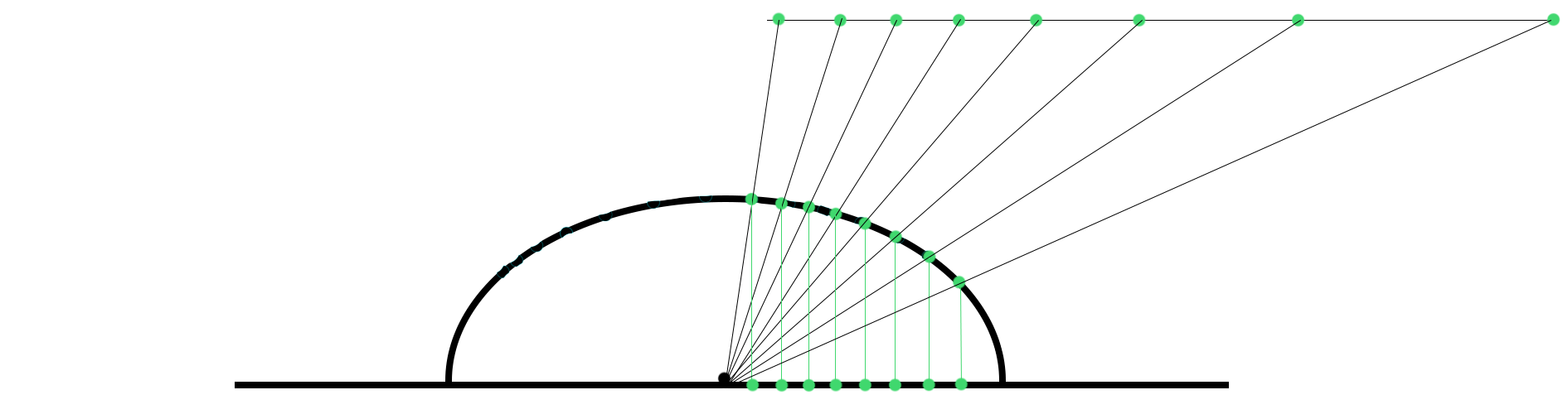
This leads to a cosine weighted distribution along the solid angle and an even more dense distribution of samples on the area light where they contribute the most. Importance sampling at its finest! Unfortunately, I’ve yet to see an implementation of this that doesn’t rely on a numerical solve so the cost of generating these samples is often quite high. We’ll stick to sampling the solid angle for now since it has lesser drawbacks.
Of course, sampling the solid angle does have some drawback. The work required to generate the samples on the solid angle is greater than what you would pay for sampling the area of the light. The reduction in variance from better sample placement is well worth this cost until the solid angle of the light becomes very small and all techniques begin to generate very similar sample directions. The typical solution for this is to calculate the solid angle and then choose which technique to use for sampling based on that.
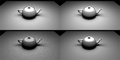
Let’s jump ahead and take a look at this in action. Based on the description above in a scene with a small rectangular area light centered directly above it we would expect both strategies to have similar noise levels directly under the light and then for the solid angle sampling to have reduced noise further away from the light. Both images below were created using 1 camera ray per pixel and 4 light rays are cast at the intersection. To show the effect of the light as clearly as possible I used a Lambertian BRDF here. On the left I used area sampling and on the right I used solid angle sampling.
You might need to click on the image to see the full-sized version in order to clearly see the difference but its behavior matches what we’d expect. Now some food for thought, if we used this same scene but with a light shape with more complicated geometry, like a sphere or a disk, how would we expect the results to change?
Sampling the solid angle of a spherical light source
Before I answer that let’s first start with how to sample the solid angle of a spherical light source. I’ll be following along with section 3.2.2 of Shirley 1996 and adding a few details for clarity.
The first step is going to be to build a basis with one axis, $\w$, facing in the direction of the sphere. Using the notation from the paper we have:
$$\w = \frac{\c - \x}{||\c - \x||}$$
$$\v = \frac{(\w \times \n)}{||\w \times \n||}$$
$$\u = \frac{\w \times \v}{||\w \times \v||}$$
where $\x$ is the origin, $\c$ is the center point of the sphere, and $\n$ is some direction that is not pointing directly at or away from $\w$. The maximum angle that includes the spherical light is given by $\thetamax$ which can be solved for by understanding that we want to find a vector through $\x$ that is orthogonal to the sphere and then using some basic trigonometry. For a clearer view of that of here is a diagram from [Wang 1993]:
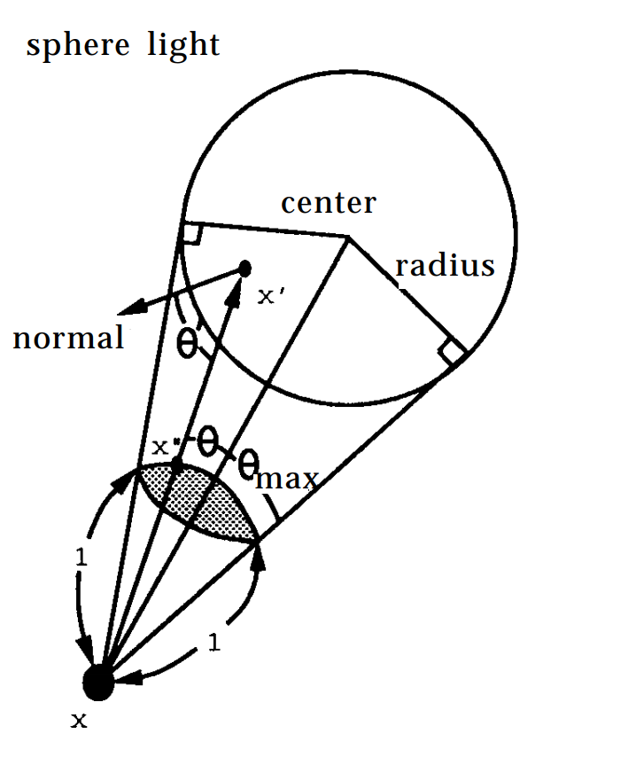
So we can see that $\thetamax$ can be calculated with some basic trigonometry on the right triangle formed by $\x$, $\c$, and the point where the vector orthogonal to the sphere hits the sphere:
$$\theta_{max} = \arcsin(\frac{\r}{||\c - \x||}) = \arccos(\sqrt{1 - (\frac{\r}{||\c - \x||})^2})$$
Since we want a uniform density on the solid angle subtended by the sphere we want to find the solid angle of the cone with apex angle $\thetamax$ and sample that uniformly. Fortunately, our friend Archimedes found that the solid angle of a cone with apex angle $2\theta$ is $\Omega = 2\pi(1-\cos\theta)$. There’s a proof for that in section 2.2 here. With that we know we want to uniformly sample with:
$$q_2(\w’) = \frac{1}{2\pi(1 - cos\thetamax)} = \frac{1}{2\pi(1 - \sqrt{1 - (\frac{\r}{||\c - \x||})^2})}$$
Now we’re going to use the same inversion method that I mentioned in my first blog post to generate the spherical coordinates of our sample. We start by converting the above equation from solid angle to spherical coordinates:
$$q_2(\theta, \phi) = \frac{\sin\theta}{2\pi(1 - \sqrt{1 - (\frac{\r}{||\c - \x||})^2})}$$
As you can see this equation is independent of $\phi$ and since $\phi$ ranges from 0 to $2\pi$ we can sample that uniformly with $\phi = 2 \pi \xi_2$ where $\xi_2$ is a random number between 0 and 1. To sample $\theta$ we calculate the CDF:
$$q_2(\theta) = \int_0^{2\pi} q_2(\theta, \phi) d\phi = \frac{\sin\theta}{1 - \sqrt{1 - (\frac{\r}{||\c - \x||})^2}}$$ $$Q_2(\theta) = \int_0^\theta q_2(t)dt = \frac{1 - \cos\theta}{1 - \sqrt{1 - (\frac{\r}{||\c - \x||})^2}}$$
Then we set that as canonical random number $\xi_1 = Q_2(\theta)$ and solve for $\theta$ to get:
$$\theta = \arccos(1 - \xi_1 + \xi_1 \sqrt{1 - (\frac{\r}{||\c - \x||})^2})$$
Ok we’re almost there. We can use coordinates $(\theta, \phi)$ to generate a direction in our default coordinate system and then use the basis defined by $\w, \v, \u$ from earlier to rotate our sample to point at the spherical light source. This gives us a direction $\a$ from $\x$ towards the spherical light. In my case with a left-handed, y-up coordinate system that is:
$$\a = \begin{bmatrix}\cos\phi\sin\theta & \cos\theta & \sin\phi\sin\theta\end{bmatrix} \begin{bmatrix}\u_x & \u_y & \u_z \\ \w_x & \w_y & \w_z \\ \v_x & \v_y & \v_z\end{bmatrix}$$
To find the point $\x’$ on the spherical area light we then perform a simple ray-sphere intersection with ray origin $\x$, direction $\a$, sphere center $\c$ and radius $\r$. I’m going to leave that out here since it’s covered in quite a few places on the internet. With the ray-sphere intersection method I used I found that I could occasionally fail the intersection test by a very small margin due to precision issues so in that case I projected the ray onto its nearest point on the sphere. Since we are importance sampling the final step we need to take is to calculate the probability of having sampled $\x’$. To calculate this I need to mention the solid angle measure:
$$d\sigma(\w’) = dA(\x’)\frac{\w’ \cdot \n’}{||\x - \x’||^2}$$
which describes the relation between differential solid angle and differential area. We can use this with our pdf $q_2(\w’)$ defined in solid angle space to find the pdf $p(\x’)$ for our sample.
$$p(\x’) = \frac{(\w’ \cdot \n’)}{2\pi ||\x - \x’||^2 (1 - \sqrt{1 - (\frac{\r}{||\c - \x||})^2})}$$
Ok… wait… what? That’s a bit confusing at first glance. Let’s think about a spherical light source whose edge is right on the unit hemisphere so that both $||\x - \x’||^2$ and $(\w’ \cdot \n’)$ are near 1. Since we’re talking in terms of differential area here we want to zoom in on an infinitely small subset of the surface so that we can think of it as being locally flat. What does the area of that surface look like? Because we’ve set this up in a pretty specific way it should be easy to see that it’s the same as its solid angle. And so the probability of sampling any particular point on this surface is the same as choosing any particular direction within that solid angle. Now let’s move the light back so that $||\x - \x’||^2 = 4$ and look at a section that covers the same solid angle. What has changed? The solid angle is the same and thus the probability of choosing any particular direction within the solid angle will remain the same as before. However, the area of this surface will have increased by a factor of 4 which means that the probabily of choosing any particular point on this surface has decreased by the same factor of 4. You can follow the same exercise to see how changing the angle of the surface effects the probability of choosing a point on the surface.
At that’s about it! If you are already familar with using area lights that is everything you need to sample with the solid angle. However, if you are new to that as well I’ll also quickly mention that the integral we want to solve as we are sampling the area light is the area form of the rendering equation given by:
$$\textit{L}_d(\x, \w) = \int _\chi \textit{g}(\x, \x’) \textit{p}(\x, \w, \w’) (-\w’ \cdot \n) \frac{(\w’ \cdot \n’)}{||\x - \x’||^2}d\textit{A}(\x’)$$
where $\textit{g}(\x, \x’)$ is either 0 or 1 depending on whether or not the shadow ray hits anything and $\textit{p}(\x, \w, \w’)$ is, of course, the BRDF. Once we’ve calculated a point $\x’$ to sample we’ll use that to calculate it’s corresponding $\w’$ and $\n’$ and plug those into this equation and then divide our sample by the probability of having chosen it. You can see that some of those terms will cancel out with the pdf I described earlier.
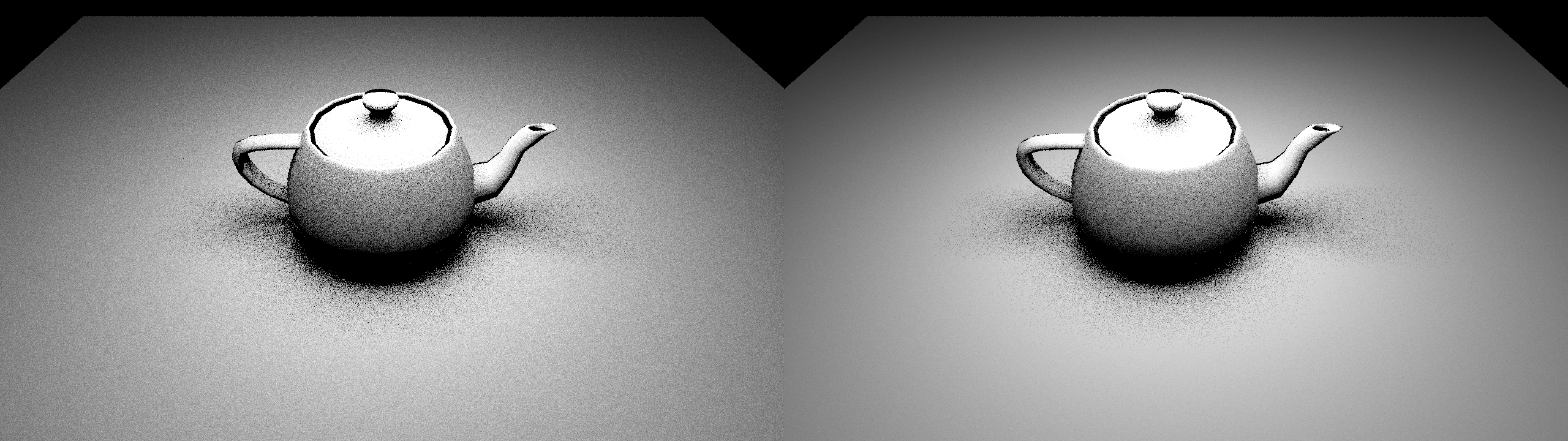
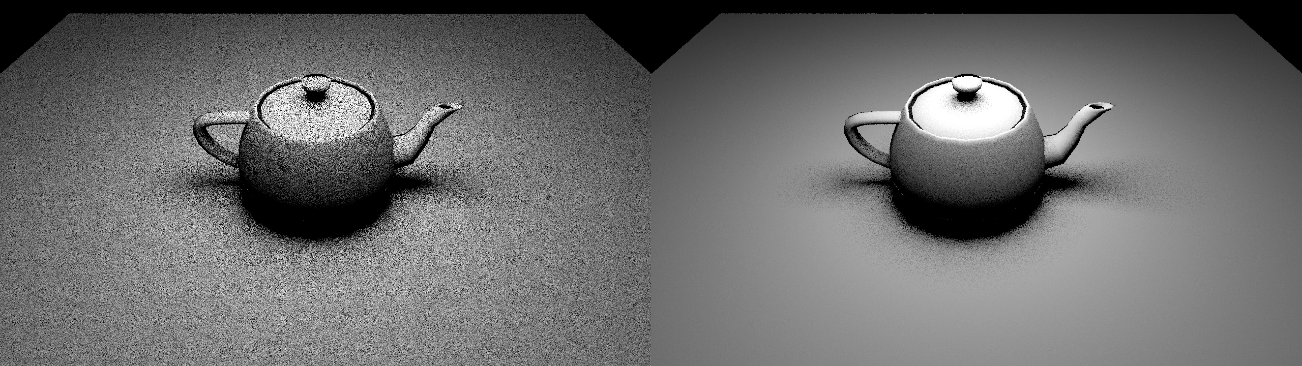
Did you think about the food for thought I left you with after the image from the first scene? I hope so because we have some spoilers right below. This is the same scene and sample counts described above except with a spherical light source. In this case we can see that solid angle sampling gives better results even directly under the light. My intuition for this is that it’s happening because as samples move away from the center of the spherical light both terms of the solid angle measure will decrease faster than they would with a rectangular light so sample placement matters even more here.
For some code showing this technique in action, look no further!
//====================================================================
static float3 IntegrateSphereLight(RTCScene& rtcScene,
                                   Random::MersenneTwister* twister,
                                   const SurfaceParameters& surface,
                                   SphericalAreaLight light,
                                   uint lightSampleCount)
{
    float3 L = light.intensity;
    float3 c = light.center;
    float  r = light.radius;

    float3 o = surface.position;

    float3 w = c - o;
    float distanceToCenter = Length(w);
    w = w * (1.0f / distanceToCenter);

    float q = Math::Sqrtf(1.0f - (r / distanceToCenter)
                               * (r / distanceToCenter));

    float3 n = surface.normal;
    float3 v, u;
    MakeOrthonormalCoordinateSystem(w, &v, &u);

    float3x3 toWorld = MakeFloat3x3(u, w, v);

    float3 Lo = float3::Zero_;

    for(uint scan = 0; scan < lightSampleCount; ++scan) {
        float r0 = Random::MersenneTwisterFloat(twister);
        float r1 = Random::MersenneTwisterFloat(twister);

        float theta = Math::Acosf(1 - r0 + r0 * q);
        float phi   = Math::TwoPi_ * r1;

        float3 local = Math::SphericalToCartesian(theta, phi);
        float3 nwp = MatrixMultiply(local, toWorld);
        float3 wp = -nwp;

        float3 xp;
        Intersection::RaySphereNearest(o, nwp, c, r, xp);

        float distSquared = LengthSquared(xp - o);
        float dist = Math::Sqrtf(distSquared);

        float dotNL = Saturate(Dot(nwp, surface.normal));
        if(dotNL > 0.0f
           && OcclusionRay(rtcScene, surface, nwp, dist)) {
            // -- the dist^2 and Dot(w', n') terms from the pdf and
            // -- the area form of the rendering equation cancel out
            float pdf_xp = 1.0f / (Math::TwoPi_ * (1.0f - q));
            Lo += dotNL * (1.0f / pdf_xp) * L;
        }
    }

    return Lo * (1.0f / lightSampleCount);
}
Sampling the solid angle of a other light shapes
There are quite a few papers now that have solved for sampling the solid angle of other light shapes. The first image I showed that sampled the solid angle of a rectangular light source used the technique from Ureña 2013. My first revision of this blog post actually went into the details of this paper as well but after it was all written up I realized I had added very few clarifications so I think that speaks very highly of how readable this paper is. They even include source code at the bottom so it has everything you need.
For sampling of spherical triangles check out Arvo 1995. This could be very useful if you want to emit light from a very complicated piece of geometry by tessellating it although stratification of samples across multiple triangles is not handled by this technique alone.
For sampling of spherical ellipses, which would include both disk and ellipsoid light shapes, check out Guillén 2017.
That’s everything for today. Thanks again for reading and feel free to leave any feedback on twitter @schuttejoe.
References:
- [Shirley 1996] Monte Carlo Techniques for Direct Lighting Calculations
- [Wang 1993] Physically Correct Direction Lighting for Distribution Ray Tracing
- [Mazonka 2012] Solid Angle of Conical Surfaces, Polyhedral Cones, and Intersecting Spherical Caps
- [Ureña 2013] An Area-Preserving Parametrization for Spherical Rectangles
- [Arvo 1995] Stratified Sampling of Spherical Triangles
- [Guillén 2017] Area-Preserving Parameterizations for Spherical Ellipses
edit 4/11/2018: fixed spelling mistake pointed out to me by @raroni86.