Importance Sampling techniques for GGX with Smith Masking-Shadowing: Part 1
March 7, 2018
Today I’ll be writing about importance sampling the GGX BRDF. GGX used with the Smith masking-shadowing function has become ubiquious in the game industry so it was the first specular model I wanted to implement in the path tracer I’m writing. About two weeks before I wrote this blog post I sat down and googled “importance sampling ggx” and while I was able to find a number of articles and papers that described specific details of the technique I was left a little unsure about whether I was combining the pieces together correctly. This blog post is a result of my investigation that followed and will hopefully provide enough details along the way that anyone in the future who searches for a similar phrase will be confident in their implementation.
Additionally, Eric Heitz and Eugene D’Eon have published some wonderful research in the last few years that made improvements on the technique which I was not able to find any mention of in other blogs so hopefully by writing about that in Part 2 of this post I am able to increase the visiblity of their improvements.
Ok let’s get started by describing the problem we want to solve. I’m pretty sure there’s a rule that you need to include the rendering equation in your first blog post. Or maybe it was something you did for good luck? Either way, I’m going to lead with that and try to make use of it.
$$\L_o(X, \wo) = \L_e(X, \wo) + \int_\Omega \L_i(X, \wi) ~ f(\wi, \wo) ~ | \wi \cdot \wg | ~ d\wi $$
When evaluating a single ray hit in a path tracer we want to zoom in on the interior of that integral. Furthermore, we know that $\L_i(X, \wi)$ will be information gathered by casting a ray in direction $\wi$ so we just want to focus here on choosing a direction $\wi$ and then solving for $f(\wi, \wo) ~ | \wi \cdot \wg |$. The equation $f(\wi, \wo)$ here is the Cook-Torrance microfacet BRDF described by:
$$\f(\wi,\wo) = \frac{\F(\wi,\wm) ~ \G_2(\wi,\wo,\wm) ~ \D(\wm)}{4 ~ |\wi\cdot\wg| ~ |\wo\cdot\wg|}$$
In our specific example we are looking at the GGX distribution of normals for $\D(\wm)$ and the Smith masking-shadowing function for $\G_2(\wi,\wo,\wm)$. These equations are written as:
$\D(\wm) = \frac{\a^2}{\pi((\wg \cdot \wm)^2(\a^2-1) + 1)^2}$
$\G_2(\wi, \wo) = \frac{2 (\wg \cdot \wi) (\wg \cdot \wo)}{ (\wg \cdot \wo) \sqrt{\a^2 + (1-\a^2)(\wg\cdot\wi)^2} + \wg \cdot \wi \sqrt{\a^2 + (1 - \a^2)(\wg \cdot \wo)^2}}$
$\D(\wm)$ is defined in Microfacet Models for Refraction through Rough Surfaces and the uncorrelated version of $\G_2(\wi, \wo)$ that we use can be found in PBR Diffuse Lighting for GGX+Smith Microsurfaces.
Now back to describing the problem we are solving. We know that we want to find $\wi$ and calculate $f(\wi, \wo) ~ | \wi \cdot \wg |$. As inputs we have a surface roughess $\a$, an outgoing direction $\wo$, and a geometric normal $\wg$ from our surface. Both of those vectors will have been transformed to tangent space so $\wg$ will actually be just our up direction. In my case, that is the Y axis. We have everything we need so let’s get started.
The first technique I want to write about is to importance sample only $\D(\wm)$. This is quite effective since the distribution of normals does have a significant impact on shape of the entire BRDF. To importance sample $\D(\wm)$ we will use the inverse of the CDF of $\D(\wm)$ to generate a microfacet normal $\wm$. If you are familar with using GGX in game rendering this can be thought of as creating a half vector in tangent space. The derivation of the inverse of the CDF is covered in detail in Cao Jaiyin’s post here so I’ll just refer you to that for the details and list the relevant equations here:
$$\theta_m = \arccos\sqrt{\frac{1 - \xi_0}{\xi(\a^2 -1) + 1}} ~ ~ ~ ~ ~ ~ ~ ~ ~\phi = 2 \pi \xi_1$$
Now, if you remember how importance sampling works, you’ll know that we are eventually going to need to divide our result by the pdf of the sample we take. As we will see the convienance of later, the pdf for generating the spherical coordinates is very similar to the distribution of normals itself. From Cao’s post we have:
$$\p(\theta_m, \phi) = \frac{\a^2\cos\theta_m\sin\theta_m}{\pi((\a^2 - 1)\cos^2\theta_m + 1)^2}$$
The next step we’ll want to take is to transform these spherical coordinates into Cartesian coordinates. I think if you are familar with everything I’ve said so far you probably already know the equations for this but I’ll list them for the sake of completeness. With one last reminder that I am using Y-up, here they are:
$$\textit{x} = \textit{r}\sin\theta\cos\phi$$ $$\textit{y} = \textit{r}\cos\theta~~~~~~~~$$ $$\textit{z} = \textit{r}\sin\theta\sin\phi$$
where r = 1 in this case. This gives us $\wm$.
Ok, let’s step aside for a moment and talk about what the transformation from spherical to Cartesian coordinates does to our pdf. Assuming we drew our sample x from a random variable X and then we apply some transformation $\textit{T}$ to that sample it can be thought of as us having drawn a sample from a different random variable Y with the property that
$$\p_y(y) = \p_y(T(x)) = \frac{\p_x(x)}{|\textit{J}_T(x)|}$$
where $|\textit{J}_\textit{T}(x)|$ is the absolute value of the determinant of the Jacobin of transformation $\T$. That’s a lot of words to describe one thing O_O. If you want even more words and to see more details of the derivation you can find that in section 3 of Notes on the Ward BRDF.
Armed now with that knowledge and given that the Jacobian of the transformation from spherical to Cartesian is given as:
$$|\textit{J}_T| = \textit{r}^2\sin\theta$$
we can divide that from the pdf $\p_m(\theta_m, \phi)$ with r still equal to 1 to see that we’ve canceled out the $sin\theta$ term. We can also now substitude in $\D(\wm)$ and write $\cos\theta$ as $(\wm \cdot \wg)$ to get:
$$\p_m(\wm) = \D(\wm)(\wm \cdot \wg)$$
We’re almost there. Now that we have our microfacet normal $\wm$ we can use that to calculate the light direction $\wi$ that we want to sample by reflecting our view vector $\wo$ by $\wm$. This is the final step for generating $\wi$ but note that we’ll be doing another transformation when we reflect the vector so we’re going to need to divide the pdf by the determinant of that Jacobian as well. The equation for reflection is given by:
$$\wi = 2|\wo \cdot \wm|\wm - \wo$$
and the determinent of the Jacobian of that transformation is given by:
$$|\textit{J}_R| = 4|\wo \cdot \wm|$$
Time for another aside. Many of you might have raised some question marks with that last equation. A number of papers will state that the determinent of the Jacobian of the reflection is $|\textit{J}_R| = \frac{1}{4|\wo \cdot \wm|}$. After some confusion followed by some more searching I’m going to give you an intuitive derivation for how I arrived at what I did. From Notes on the Ward BRDF we get this diagram:
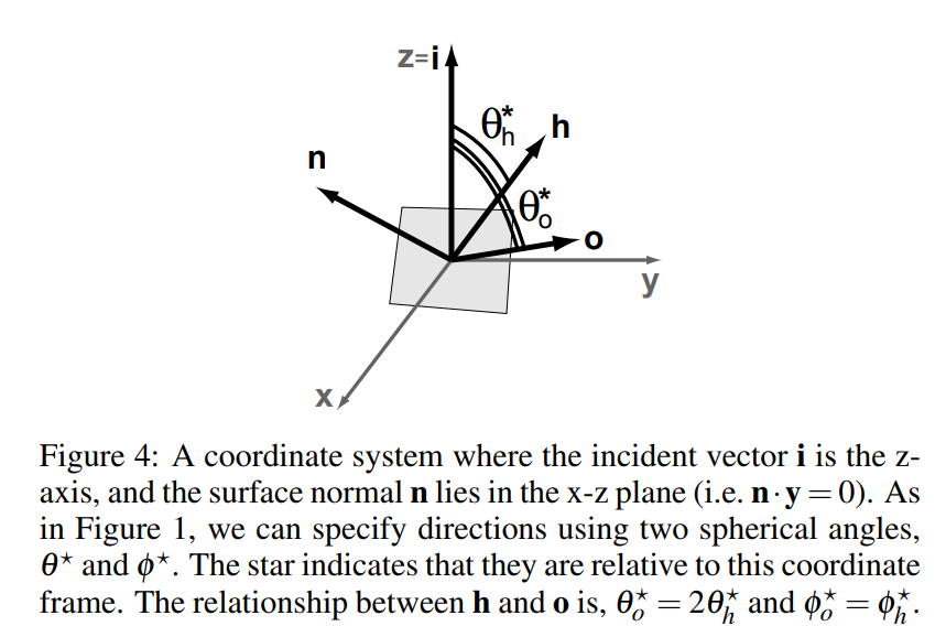
Using Wards notation for a generic set of vectors $\textit{i}$, $\textit{h}$, and $\textit{n}$ what we want to do is:
- Rotate the vectors to have the orientation described in Ward’s image. This has a Jacobian of 1 since rotation is a linear transform.
- Transform the vector into spherical coordinates. This has a Jacobian of $\frac{1}{\sin\theta_h}$.
- Apply the transform $f(\theta_h, \phi_h) = (2\theta_h, \phi_h) = (\theta_o, \phi_h)$. This has a Jacobian of 2.
- Transform the new coordinates back to Cartesian coordinates. This has a Jacobian of $\sin\theta_o$.
- Perform the inverse rotation from our first step. This has a Jacobian of 1 again.
Now we have calculated the reflected vector $\textit{o}$ in a far more complicated way than we described earlier but this now has much easier steps for deriving the Jacobian. Since the Jacobian of the composition of two transformations is just the product of those two Jacobians we just need to multiply the above Jacobians together. This gives us:
$$|\frac{2\sin\theta_o}{\sin\theta_h}| = |\frac{2\sin(2\theta_h)}{\sin\theta_h}| = |\frac{4\sin\theta_h\cos\theta_h}{\sin\theta_h}| = 4|cos\theta_h|$$
Ah, well, there it is.
All right, back on topic. When we now take that Jacobian and divide that out from $\p_m(\wm)$ we get the final pdf for sampling $\wi$. I’m going to play a little fast and loose with notation here and call it $\p_i(\wm, \wo)$
$$\p_i(\wm, \wo) = \frac{\D(\wm)(\wm \cdot \wg)}{4|\wo \cdot \wm|}$$
Now that we have direction $\wi$ and the pdf of the random variable that generated $\wi$ we have everything we need to solve for the reflectance. We now take the $f(\wi, \wo) ~ |\wi \cdot \wg |$ term we mentioned at the beginning and divide that by the pdf $\p_i(\wm, \wo)$ to solve for the reflectance coming from direction $\wi$.
$$\frac{\f(\wi,\wo)| \wi \cdot \wg |}{\p_i(\wm, \wo)} = \frac{\frac{\F(\wi,\wm) ~ \G_2(\wi,\wo,\wm) ~ \D(\wm)| \wi \cdot \wg |}{4 ~ |\wi\cdot\wg| ~ |\wo\cdot\wg|}}{\frac{\D(\wm)(\wm \cdot \wg)}{4|\wo \cdot \wm|}}$$ $$= \frac{\F(\wi,\wm) ~ \G_2(\wi,\wo,\wm) ~ \D(\wm)| \wi \cdot \wg |}{4 ~ |\wi\cdot\wg| ~ |\wo\cdot\wg|} * \frac{4|\wo \cdot \wm|}{\D(\wm)(\wm \cdot \wg)}$$
Conveniently you can see that a few terms cancel out and we’re left with only this for our reflectance:
$$\frac{\f(\wi,\wo)| \wi \cdot \wg |}{\p_i(\wm)} = \boxed{\frac{\F(\wi,\wm) \G_2(\wi,\wo,\wm) |\wo \cdot \wm|}{|\wo \cdot \wg| |\wm\cdot\wg|}}$$
From here we will transform $\wi$ from the tangent space we’ve been working in back to world space, cast a ray in that direction to solve for incoming energy $\L_i(X, \wi)$, and multiply that by the reflectance we calculated here.
Now let’s look at the results!
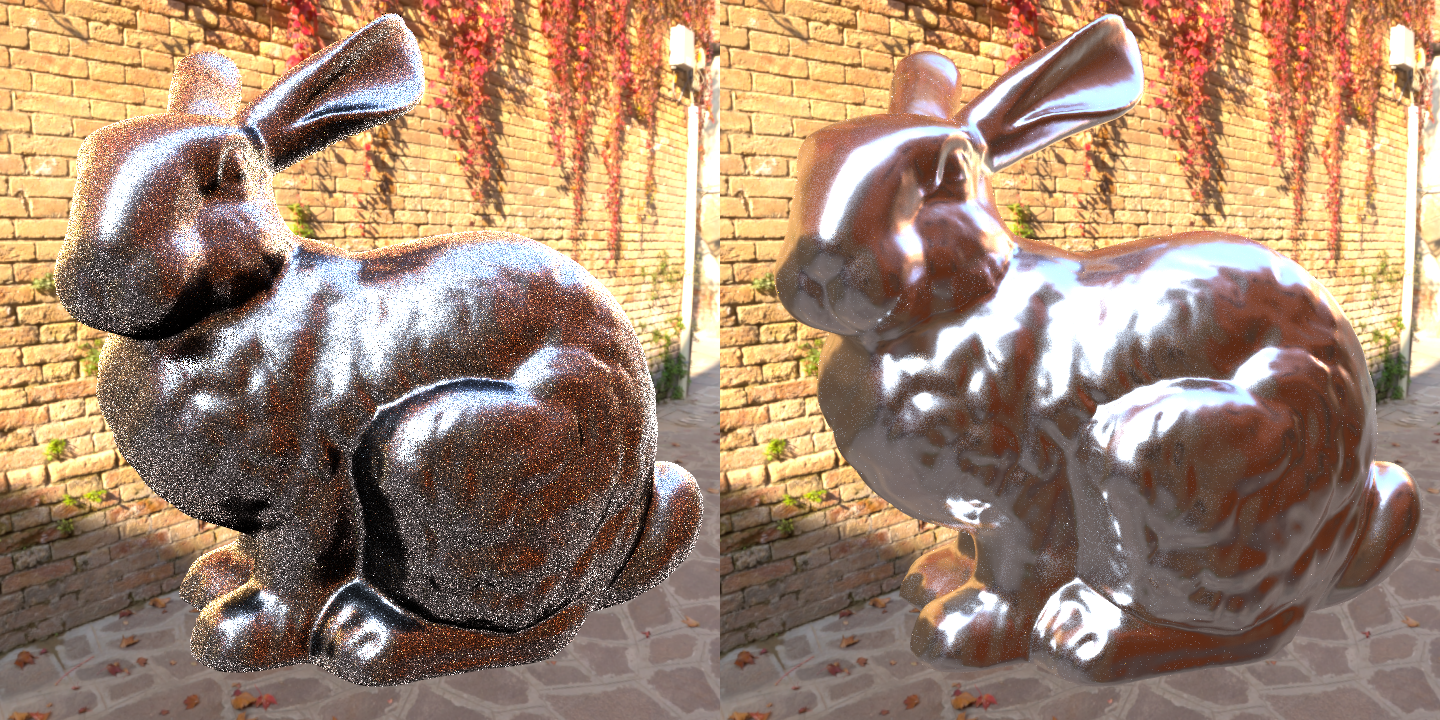
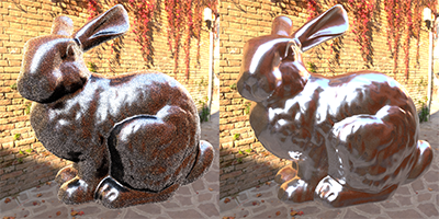
In order to have something to compare to on the left I generated an image by importance sampling a cosine distribution and on the right I generated an image using the technique described above. The scene is the Stanford bunny with roughness 0.05 lit only with an environment light. Both images were generated with 512 rays per pixel.
As you can see the results are significantly higher quality than importance sampling with just a cosine lobe. However, there are still quite a few fireflys visible in the image so this technique would require a lot more samples to converge. In my next post I will talk about why we still see so many fireflys and about a more recent technique from Eric Heitz and Eugene D’Eon to importance sample the distribution of visible normals that fixes some of these problems.
One last thing before we move on to part 2 is I want to provide source code to help ground all of this. You’ll need to fill in some blanks but the key parts are covered here.
//====================================================================
static float3 SchlickFresnel(float3 r0, float radians)
{
    // -- The common Schlick Fresnel approximation
    float exponential = Powf(1.0f - radians, 5.0f);
    return r0 + (1.0f - r0) * exponential;
}

//====================================================================
// non height-correlated masking-shadowing function is described here:
static float SmithGGXMaskingShadowing(float3 wi, float3 wo, float a2)
{
    float dotNL = BsdfNDot(wi);
    float dotNV = BsdfNDot(wo);

    float denomA = dotNV * Sqrtf(a2 + (1.0f - a2) * dotNL * dotNL);
    float denomB = dotNL * Sqrtf(a2 + (1.0f - a2) * dotNV * dotNV);

    return 2.0f * dotNL * dotNV / (denomA + denomB);
}

//====================================================================
void ImportanceSampleGgxD(Random::MersenneTwister* twister, float3 wg,
                          float3 wo, Material* material,
                          float3& wi, float3& reflectance)
{
    float a = material->roughness;
    float a2 = a * a;

    // -- Generate uniform random variables between 0 and 1
    float e0 = Random::MersenneTwisterFloat(twister);
    float e1 = Random::MersenneTwisterFloat(twister);

    // -- Calculate theta and phi for our microfacet normal wm by
    // -- importance sampling the Ggx distribution of normals
    float theta = Acosf(Sqrtf((1.0f - e0) / ((a2 - 1.0f) * e0 + 1.0f)));
    float phi   = Math::TwoPi_ * e1;

    // -- Convert from spherical to Cartesian coordinates
    float3 wm = Math::SphericalToCartesian(theta, phi);

    // -- Calculate wi by reflecting wo about wm
    wi = 2.0f * Dot(wo, wm) * wm - wo;

    // -- Ensure our sample is in the upper hemisphere
    // -- Since we are in tangent space with a y-up coordinate
    // -- system BsdfNDot(wi) simply returns wi.y
    if(BsdfNDot(wi) > 0.0f && Dot(wi, wm) > 0.0f) {

    	float dotWiWm = Dot(wi, wm);

        // -- calculate the reflectance to multiply by the energy
        // -- retrieved in direction wi
        float3 F = SchlickFresnel(material->specularColor, dotWiWm);
        float G = SmithGGXMaskingShadowing(wi, wo, a2);
        float weight = Absf(Dot(wo, wm))
                     / (BsdfNDot(wo) * BsdfNDot(wm));

        reflectance = F * G * weight;
    }
    else {
        reflectance = float3::Zero_;
    }
}
And that’s it for today. For a description of the flaws with this method and a writeup about an even better method see part 2 of this post. Thanks for reading!
(Edit 3/12/18: I found an error in the Smith masking shadowing equation and function and corrected it.)
References:
- Microfacet Models for Refraction through Rough Surfaces
- PBR Diffuse Lighting for GGX+Smith Microsurfaces
- Sampling microfacet BRDF
- Notes on the Ward BRDF
Additional thanks to:
- HDRI Haven for the free IBL
- My friends who helped review this. Special credit to Matt Pettineo for providing a link to the Ward paper.
While I had an absolute blast writing this series and I definitely want to write more in the future I’m waiting to gague reactions before I decide how much sense it makes to put effort into the appearance of the site. Until I decide to flesh things out more you can leave comments at: