Rendering the Moana Island Scene Part 1: Implementing the Disney BSDF
August 10, 2018
$\newcommand{\i}{\textit{i}}$ $\newcommand{\o}{\textit{o}}$ $\newcommand{\n}{\textit{n}}$ $\newcommand{\h}{\textit{h}}$ $\newcommand{\v}{\textit{v}}$ $\newcommand{\x}{\textit{x}}$ $\newcommand{\y}{\textit{y}}$ $\newcommand{\ht}{\textit{h}_t}$
Intro
The Disney BRDF was introduced by Brent Burley as part of the SIGGRAPH 2012 Physically Based Shading course and then extended to a BSDF with integrated subsurface scattering for the SIGGRAPH 2015 Physically Based Shading course. While the model is not strictly physically based it was designed with physically based principles in mind and each of the terms included was done so to fit the model to materials in the MERL 100 database. More importantly, each term was carefully chosen and parameterized to be easy for artists to use and so that blending multiple layers together would give intuitive results. I believe it is these later traits that have made the Disney BSDF to be so successful.
The materials in the Moana Island scene are all one of two types: “solid” or “thin”. Both material types generally behave the same with the exception being when transmission is involved. For thin materials there is no internal surface so subsurface scattering is approximated with Hanrahan-Krueger diffuse. Additionally, since there is also no volume to refract into and later out of both the enter and exit events are modeled simultaneously at the same point. The most common example of this material type in the Island scene is for leaves and other foliage modeled without an interior volume. It would then make sense to guess that the solid material type is for objects that are modeled with an interior volume.
The title of my blog (Rendering Equations) wouldn’t be a bad pun for giving you a bunch of equations if I didn’t include a whole bunch of equations in each post. So next I’ll describe each individual lobe of the Disney BSDF and then I’ll wrap up by discussing sampling of each lobe.
Sheen
The sheen lobe is probably the simplest of all of the terms so we’ll start here. It is a standalone lobe that is added to the others based on a $\textit{sheen}$ parameter with its color varying between white and the a tinted color depending on the $\textit{sheenTint}$ parameter. It’s purpose is to model light at grazing angles on a surface so it will mostly be used for retro-reflection seen in cloth or on rougher surfaces to add back in energy lost due to a geometry term that only models single-scattering. I wouldn’t be surprised to see this term be replaced with something like Multiple-Scattering Microfacet BSDFs with the Smith Model or A Multi-Faceted Exploration (Part 2) in Disney’s future iterations though that would necessitate an alternate solution for retro-reflection where their diffuse term is insufficient.
While I don’t recall seeing it mentioned anywhere in the notes, in the Disney BRDF Explorer they extract the hue and saturation from the base color and use that for the sheen lobe’s tint color rather than using the base color directly. This is done by calculating the luminance using approximate, linear-space CIE luminance weights and then normalizing:
static float3 CalculateTint(float3 baseColor)
{
    // -- The color tint is never mentioned in the SIGGRAPH presentations as far as I recall but it was done in
    // --  the BRDF Explorer so I'll replicate that here.
    float luminance = Dot(float3(0.3f, 0.6f, 1.0f), baseColor);
    return (luminance > 0.0f) ? baseColor * (1.0f / luminance) : float3::One_;
}
With that we can then calculate the intensity of the sheen lobe: $$f(\textit{sheen}, \theta_d) = \textit{sheen} * ((1 - \textit{sheenTint}) + \textit{sheenTint} * \textit{tint}) * (1 - \cos\theta_d)^5$$
static float3 EvaluateSheen(const SurfaceParameters& surface, const float3& wo, const float3& wm, const float3& wi)
{
    if(surface.sheen <= 0.0f) {
        return float3::Zero_;
    }

    float dotHL = Dot(wm, wi);
    float3 tint = CalculateTint(surface.baseColor);
    return surface.sheen * Lerp(float3(1.0f), tint, surface.sheenTint) * Fresnel::SchlickWeight(dotHL);
}
Clearcoat
The Clearcoat lobe is another additive lobe that is controlled by a $\textit{clearcoat}$ parameter for its intensity and a $\textit{clearcoatGloss}$ parameter for its shape. This lobe is a bit more complicated and models a full BRDF but most of its terms are fixed to keep this lobe as a simple, artist-friendly way to model, well, a clear… coating on top of a material. It’s pretty well named.
The distribution term used for the clearcoat layer is a fixed form of a BRDF created by Burley and called Generalized Trowbridge-Reitz. Here is its normalized form with a fixed gamma of one used for clearcoat via Burley’s course notes:
$$D_{GTR_1}(x) = \frac{\alpha^2 - 1}{\pi\log(\alpha^2)} \frac{1}{1 + (\alpha^2 - 1)\cos^2\theta_h}$$
The Fresnel term uses the Schlick approximation with a fixed index of refraction of 1.5 to be representative of polyurethane. This evaluates to $F_0 = 0.04$. If you want details on how that is calculated Sébastien Lagarde wrote about the Fresnel equation in a ton of detail.
$$f_{Schlick} = F_0 + (1 - F_0)(1 - \cos\theta_h)^5$$
The masking-shadowing term used was the separable form of Smith for GGX with a fixed roughness of 0.25. While the term is not the correct match for the distribution of normals as of the 2014 addendum to the 2012 course notes it looks like they were happy with the look and have not changed it.
$$G(\theta, \alpha) = \frac{1}{\cos\theta + \sqrt{\alpha^2 + \cos\theta - \alpha^2\cos^2\theta}}$$ $$G(\theta_l, \theta_v) = G(\theta_l, 0.25) * G(\theta_v, 0.25)$$
//===================================================================================================================
static float GTR1(float absDotHL, float a)
{
    if(a >= 1) {
        return InvPi_;
    }

    float a2 = a * a;
    return (a2 - 1.0f) / (Pi_ * Log2(a2) * (1.0f + (a2 - 1.0f) * absDotHL * absDotHL));
}

//===================================================================================================================
float SeparableSmithGGXG1(const float3& w, float a)
{
    float a2 = a * a;
    float absDotNV = AbsCosTheta(w);

    return 2.0f / (1.0f + Math::Sqrtf(a2 + (1 - a2) * absDotNV * absDotNV));
}

//===================================================================================================================
static float EvaluateDisneyClearcoat(float clearcoat, float alpha, const float3& wo, const float3& wm,
                                     const float3& wi, float& fPdfW, float& rPdfW)
{
    if(clearcoat <= 0.0f) {
        return 0.0f;
    }

    float absDotNH = AbsCosTheta(wm);
    float absDotNL = AbsCosTheta(wi);
    float absDotNV = AbsCosTheta(wo);
    float dotHL = Dot(wm, wi);

    float d = GTR1(absDotNH, Lerp(0.1f, 0.001f, alpha));
    float f = Fresnel::Schlick(0.04f, dotHL);
    float gl = Bsdf::SeparableSmithGGXG1(wi, 0.25f);
    float gv = Bsdf::SeparableSmithGGXG1(wo, 0.25f);

    fPdfW = d / (4.0f * absDotNL);
    rPdfW = d / (4.0f * absDotNV);

    return 0.25f * clearcoat * d * f * gl * gv;
}
Specular BRDF
The specular BRDF is the traditional Cook-Torrance microfacet BRDF that uses Anisotropic GGX (aka GTR2) with a Smith masking-shadowing function. Burley calculated the anisotropic weights $\alpha_x$ and $\alpha_y$ with:
$$\textit{aspect} = \sqrt{1 - 0.9 * \textit{anisotropic}}$$ $$\alpha_x = \textit{roughness}^2 / \textit{aspect}$$ $$\alpha_y = \textit{roughness}^2 * \textit{aspect}$$
The anisotropic distribution of normals is:
$$D_{GTR_2aniso} = \frac{1}{\pi \alpha_x \alpha_y} \frac{1}{(\frac{(\h \cdot \x)^2}{\alpha_x^2} + \frac{(\h \cdot \y)^2}{\alpha_y^2} + (\h \cdot \n)^2)^2}$$
Via the 2014 addendum to the course notes we know that Disney changed their geometry term to match the anisotropic Smith GGX term derived by Heitz in Understanding the Masking-Shadowing Function in Microfacet-Based BRDFs.
$$G1_{GTR_2aniso} = \frac{1}{1 + \Lambda(\wo)}$$ $$\Lambda(\wo) = \frac{-1 + \sqrt{1 + \frac{1}{a^2}}}{2}$$ $$a = \frac{1}{\tan\theta_o\sqrt{\cos^2\phi_o\alpha_x^2 + \sin^2\phi_o\alpha_y^2}}$$
In the code you can see I call the DisneyFresnel function to calculate the Fresnel term. I’ll talk more about that later.
//===================================================================================================================
float GgxAnisotropicD(const float3& wm, float ax, float ay)
{
    float dotHX2 = Square(wm.x);
    float dotHY2 = Square(wm.z);
    float cos2Theta = Cos2Theta(wm);
    float ax2 = Square(ax);
    float ay2 = Square(ay);

    return 1.0f / (Math::Pi_ * ax * ay * Square(dotHX2 / ax2 + dotHY2 / ay2 + cos2Theta));
}

//===================================================================================================================
float SeparableSmithGGXG1(const float3& w, const float3& wm, float ax, float ay)
{
    float dotHW = Dot(w, wm);
    if (dotHW <= 0.0f) {
        return 0.0f;
    }

    float absTanTheta = Absf(TanTheta(w));
    if(IsInf(absTanTheta)) {
        return 0.0f;
    }

    float a = Sqrtf(Cos2Phi(w) * ax * ax + Sin2Phi(w) * ay * ay);
    float a2Tan2Theta = Square(a * absTanTheta);

    float lambda = 0.5f * (-1.0f + Sqrtf(1.0f + a2Tan2Theta));
    return 1.0f / (1.0f + lambda);
}

//===================================================================================================================
static float3 EvaluateDisneyBRDF(const SurfaceParameters& surface, const float3& wo, const float3& wm,
                                 const float3& wi, float& fPdf, float& rPdf)
{
    fPdf = 0.0f;
    rPdf = 0.0f;

    float dotNL = CosTheta(wi);
    float dotNV = CosTheta(wo);
    if(dotNL <= 0.0f || dotNV <= 0.0f) {
        return float3::Zero_;
    }

    float ax, ay;
    CalculateAnisotropicParams(surface.roughness, surface.anisotropic, ax, ay);

    float d = Bsdf::GgxAnisotropicD(wm, ax, ay);
    float gl = Bsdf::SeparableSmithGGXG1(wi, wm, ax, ay);
    float gv = Bsdf::SeparableSmithGGXG1(wo, wm, ax, ay);

    float3 f = DisneyFresnel(surface, wo, wm, wi);

    Bsdf::GgxVndfAnisotropicPdf(wi, wm, wo, ax, ay, fPdf, rPdf);
    fPdf *= (1.0f / (4 * AbsDot(wo, wm)));
    rPdf *= (1.0f / (4 * AbsDot(wi, wm)));

    return d * gl * gv * f / (4.0f * dotNL * dotNV);
}
You’ll notice that in SeparableSmithGGXG1 I use a lot of trig functions (ex: Sin2Phi, TanTheta). I’m using the unoptimized implementation described in Understanding the Masking-Shadowing Function in Microfacet-Based BRDFs. There exists an optimized form of this in the Disney BRDF explorer but that goes to infinity under some circumstances so I’m not convinced it’s correct.
Specular BSDF
The specular BSDF is an extension of the specular BRDF to handle refraction. Since I haven’t discussed refraction in this blog I’ll note that the microfacet form for it is given by:
$$f_t(\i,\o,\n) = \frac{|\i \cdot \ht|}{|\i \cdot \n|}\frac{|o \cdot \ht|}{|\o \cdot \n|}\frac{\eta^2}{(\i \cdot \ht + \eta\o\cdot\ht)^2}\frac{1}{\eta^2} (1 - F(\i, \ht)) G(\i,\o,\ht) D(\ht)$$
with $\ht = -\frac{\i + \eta\o}{||i + \eta\o||}$ and $\eta = \frac{\eta_i}{\eta_o}$ being the relative index of refraction.
Other than that, the BSDF uses the same distribution and geometry terms as the BRDF. They model the full dielectric Fresnel equation for this since they ran into issues where the relative IOR was close to 1. My implementation for Fresnel::Dielectric is just copied from PBRT so I’ll link that here rather than inline the code.
Finally, when using the thin material model we use the square root of the base color to model both the entrance and the exit event at the same time. We also adjust the anisotropic roughness parameters based on the index of refraction which is handled outside of EvaluateDisneySpecTransmission.
//===================================================================================================================
static float ThinTransmissionRoughness(float ior, float roughness)
{
    // -- Disney scales by (.65 * eta - .35) based on figure 15 of the 2015 PBR course notes. Based on their figure
    // -- the results match a geometrically thin solid fairly well.
    return Saturate((0.65f * ior - 0.35f) * roughness);
}

//===================================================================================================================
static float3 EvaluateDisneySpecTransmission(const SurfaceParameters& surface, const float3& wo, const float3& wm,
                                             const float3& wi, float ax, float ay, bool thin)
{
    float relativeIor = surface.relativeIOR;
    float n2 = relativeIor * relativeIor;

    float absDotNL = AbsCosTheta(wi);
    float absDotNV = AbsCosTheta(wo);
    float dotHL = Dot(wm, wi);
    float dotHV = Dot(wm, wo);
    float absDotHL = Absf(dotHL);
    float absDotHV = Absf(dotHV);

    float d = Bsdf::GgxAnisotropicD(wm, ax, ay);
    float gl = Bsdf::SeparableSmithGGXG1(wi, wm, ax, ay);
    float gv = Bsdf::SeparableSmithGGXG1(wo, wm, ax, ay);

    float f = Fresnel::Dielectric(dotHV, 1.0f, 1.0f / surface.relativeIOR);

    float3 color;
    if(thin)
        color = Sqrt(surface.baseColor);
    else
        color = surface.baseColor;

    // Note that we are intentionally leaving out the 1/n2 spreading factor since for VCM we will be evaluating
    // particles with this. That means we'll need to model the air-[other medium] transmission if we ever place
    // the camera inside a non-air medium.
    float c = (absDotHL * absDotHV) / (absDotNL * absDotNV);
    float t = (n2 / Square(dotHL + relativeIor * dotHV));
    return color * c * t * (1.0f - f) * gl * gv * d;
}
Diffuse BRDF
The diffuse lobe is a bit more complicated than the typical Lambert diffuse model. Burley did a lot here to fit materials to the MERL database. Their model includes both a diffuse Fresnel factor as well as a term for diffuse retro-reflection. Additionally, the non-directional portion of the model is split out such that it can be replaced with a subsurface model using either diffusion or volumetric scattering. The whole diffuse lobe is given as:
$$f_d = f_{Lambert} (1 - 0.5F_L)(1 - 0.5F_V) + f_{retro-reflection}$$
with:
$$f_{retro-reflection} = \frac{baseColor}{\pi} R_R(F_L + F_V + F_LF_V(R_R - 1))$$ $$F_L = (1 - \cos\theta_l)^5$$ $$F_v = (1 - \cos\theta_v)^5$$ $$R_R = 2 * \textit{roughness} * \cos^2(\theta_d)$$
and $f_{Lambert}$ being either a simple Lambert term:
$$f_{Lambert} = \frac{\textit{baseColor}}{\pi}$$
or, when we’re evaluating a thin surface, it will be a blend between Lambert and the Hanrahan Krueger diffuse model based on the flatness parameter.
//===================================================================================================================
static float EvaluateDisneyDiffuse(const SurfaceParameters& surface, const float3& wo, const float3& wm,
                                   const float3& wi, bool thin)
{
    float dotNL = AbsCosTheta(wi);
    float dotNV = AbsCosTheta(wo);

    float fl = Fresnel::SchlickWeight(dotNL);
    float fv = Fresnel::SchlickWeight(dotNV);

    float hanrahanKrueger = 0.0f;

    if(thin && surface.flatness > 0.0f) {
        float roughness = surface.roughness * surface.roughness;

        float dotHL = Dot(wm, wi);
        float fss90 = dotHL * dotHL * roughness;
        float fss = Lerp(1.0f, fss90, fl) * Lerp(1.0f, fss90, fv);

        float ss = 1.25f * (fss * (1.0f / (dotNL + dotNV) - 0.5f) + 0.5f);
        hanrahanKrueger = ss;
    }

    float lambert = 1.0f;
    float retro = EvaluateDisneyRetroDiffuse(surface, wo, wm, wi);
    float subsurfaceApprox = Lerp(lambert, hanrahanKrueger, thin ? surface.flatness : 0.0f);

    return InvPi_ * (retro + subsurfaceApprox * (1.0f - 0.5f * fl) * (1.0f - 0.5f * fv));
}
Bringing it all together
Now let’s describe how these terms are all brought together. The clearcoat lobe and the sheen lobe are both additive. The rest of the terms are described with this diagram from the 2015 PBR paper.
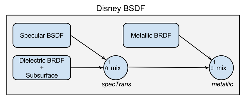
In this diagram you can see that we blend between the specular transmission lobe and the dielectric BRDF based on the specTrans parameter and then we blend that with the metallic lobe based on the metallic parameter. But what are the metallic and dielectric BRDFs in terms of the lobes I’ve described so far? The metallic BRDF uses the specular BRDF lobe with the Schlick Fresnel term with the baseColor as R0. The dielectric BRDF is a combination of the Diffuse lobe with the Specular BRDF lobe where the specular BRDF lobe uses the dielectric Fresnel equation. So what we end up with will be the specular part of both the dielectric BRDF and the metallic BRDF being evaluated with one function call and the DisneyFresnel function doing the work of blending between the two based on the metallic and specularTint surface parameters.
//===================================================================================================================
static float3 DisneyFresnel(const SurfaceParameters& surface, const float3& wo, const float3& wm, const float3& wi)
{
    float dotHV = Absf(Dot(wm, wo));

    float3 tint = CalculateTint(surface.baseColor);

    // -- See section 3.1 and 3.2 of the 2015 PBR presentation + the Disney BRDF explorer (which does their
    // -- 2012 remapping rather than the SchlickR0FromRelativeIOR seen here but they mentioned the switch in 3.2).
    float3 R0 = Fresnel::SchlickR0FromRelativeIOR(surface.relativeIOR) * Lerp(float3(1.0f), tint,
                                                                              surface.specularTint);
           R0 = Lerp(R0, surface.baseColor, surface.metallic);

    float dielectricFresnel = Fresnel::Dielectric(dotHV, 1.0f, surface.ior);
    float3 metallicFresnel = Fresnel::Schlick(R0, Dot(wi, wm));

    return Lerp(float3(dielectricFresnel), metallicFresnel, surface.metallic);
}
Now we have everything to evaluate a single surface interaction.
//===================================================================================================================
float3 EvaluateDisney(const SurfaceParameters& surface, float3 v, float3 l, bool thin,
                      float& forwardPdf, float& reversePdf)
{
    float3 wo = Normalize(MatrixMultiply(v, surface.worldToTangent));
    float3 wi = Normalize(MatrixMultiply(l, surface.worldToTangent));
    float3 wm = Normalize(wo + wi);

    float dotNV = CosTheta(wo);
    float dotNL = CosTheta(wi);

    float3 reflectance = float3::Zero_;
    forwardPdf = 0.0f;
    reversePdf = 0.0f;

    float pBRDF, pDiffuse, pClearcoat, pSpecTrans;
    CalculateLobePdfs(surface, pBRDF, pDiffuse, pClearcoat, pSpecTrans);

    float3 baseColor = surface.baseColor;
    float metallic = surface.metallic;
    float specTrans = surface.specTrans;
    float roughness = surface.roughness;

    // calculate all of the anisotropic params
    float ax, ay;
    CalculateAnisotropicParams(surface.roughness, surface.anisotropic, ax, ay);

    float diffuseWeight = (1.0f - metallic) * (1.0f - specTrans);
    float transWeight   = (1.0f - metallic) * specTrans;

    // -- Clearcoat
    bool upperHemisphere = dotNL > 0.0f && dotNV > 0.0f;
    if(upperHemisphere && surface.clearcoat > 0.0f) {

        float forwardClearcoatPdfW;
        float reverseClearcoatPdfW;

        float clearcoat = EvaluateDisneyClearcoat(surface.clearcoat, surface.clearcoatGloss, wo, wm, wi,
                                                  forwardClearcoatPdfW, reverseClearcoatPdfW);
        reflectance += float3(clearcoat);
        forwardPdf += pClearcoat * forwardClearcoatPdfW;
        reversePdf += pClearcoat * reverseClearcoatPdfW;
    }

    // -- Diffuse
    if(diffuseWeight > 0.0f) {
        float forwardDiffusePdfW = AbsCosTheta(wi);
        float reverseDiffusePdfW = AbsCosTheta(wo);
        float diffuse = EvaluateDisneyDiffuse(surface, wo, wm, wi, thin);

        float3 sheen = EvaluateSheen(surface, wo, wm, wi);

        reflectance += diffuseWeight * (diffuse * surface.baseColor + sheen);

        forwardPdf += pDiffuse * forwardDiffusePdfW;
        reversePdf += pDiffuse * reverseDiffusePdfW;
    }

    // -- transmission
    if(transWeight > 0.0f) {

        // Scale roughness based on IOR (Burley 2015, Figure 15).
        float rscaled = thin ? ThinTransmissionRoughness(surface.ior, surface.roughness) : surface.roughness;
        float tax, tay;
        CalculateAnisotropicParams(rscaled, surface.anisotropic, tax, tay);

        float3 transmission = EvaluateDisneySpecTransmission(surface, wo, wm, wi, tax, tay, thin);
        reflectance += transWeight * transmission;

        float forwardTransmissivePdfW;
        float reverseTransmissivePdfW;
        Bsdf::GgxVndfAnisotropicPdf(wi, wm, wo, tax, tay, forwardTransmissivePdfW, reverseTransmissivePdfW);

        float dotLH = Dot(wm, wi);
        float dotVH = Dot(wm, wo);
        forwardPdf += pSpecTrans * forwardTransmissivePdfW / (Square(dotLH + surface.relativeIOR * dotVH));
        reversePdf += pSpecTrans * reverseTransmissivePdfW / (Square(dotVH + surface.relativeIOR * dotLH));
    }

    // -- specular
    if(upperHemisphere) {
        float forwardMetallicPdfW;
        float reverseMetallicPdfW;
        float3 specular = EvaluateDisneyBRDF(surface, wo, wm, wi, forwardMetallicPdfW, reverseMetallicPdfW);

        reflectance += specular;
        forwardPdf += pBRDF * forwardMetallicPdfW / (4 * AbsDot(wo, wm));
        reversePdf += pBRDF * reverseMetallicPdfW / (4 * AbsDot(wi, wm));
    }

    reflectance = reflectance * Absf(dotNL);

    return reflectance;
}
Sampling
Yikes! We’re not even done yet. Evaluation of the BRDF is only half the battle; we also need to be able to sample the surface. Before we can start sampling a lobe we first need to start by choosing which lobe to sample. We can skip sheen since its intensity is relatively weak in comparison to the other lobes but that leaves us with clearcoat, specular BRDF, specular BSDF, and diffuse lobes to choose from. None of the Disney papers I’ve seen have gone into details about how this was done so I just hacked something together that assigns importance to each lobe that is proportional to the perceived intensity. This is probably bad and will likely change once I start to optimize with the full island rendering.
//===================================================================================================================
static void CalculateLobePdfs(const SurfaceParameters& surface,
                              float& pSpecular, float& pDiffuse, float& pClearcoat, float& pSpecTrans)
{
    float metallicBRDF   = surface.metallic;
    float specularBSDF   = (1.0f - surface.metallic) * surface.specTrans;
    float dielectricBRDF = (1.0f - surface.specTrans) * (1.0f - surface.metallic);

    float specularWeight     = metallicBRDF + dielectricBRDF;
    float transmissionWeight = specularBSDF;
    float diffuseWeight      = dielectricBRDF;
    float clearcoatWeight    = 1.0f * Saturate(surface.clearcoat);

    float norm = 1.0f / (specularWeight + transmissionWeight + diffuseWeight + clearcoatWeight);

    pSpecular  = specularWeight     * norm;
    pSpecTrans = transmissionWeight * norm;
    pDiffuse   = diffuseWeight      * norm;
    pClearcoat = clearcoatWeight    * norm;
}
And now sampling is relatively straightforward. I already wrote a blog post about sampling the specular BRDF though some care needs to be taken when using the thin material mode.
//===================================================================================================================
static void SampleDisneySpecTransmission(CSampler* sampler, const SurfaceParameters& surface, float3 v, bool thin,
                                         BsdfSample& sample)
{
    float3 wo = MatrixMultiply(v, surface.worldToTangent);
    if(CosTheta(wo) == 0.0) {
        sample.forwardPdfW = 0.0f;
        sample.reversePdfW = 0.0f;
        sample.reflectance = float3::Zero_;
        sample.wi = float3::Zero_;
        return false;
    }

    // -- Scale roughness based on IOR
    float rscaled = thin ? ThinTransmissionRoughness(surface.ior, surface.roughness) : surface.roughness;

    float tax, tay;
    CalculateAnisotropicParams(rscaled, surface.anisotropic, tax, tay);

    // -- Sample visible distribution of normals
    float r0 = sampler->UniformFloat();
    float r1 = sampler->UniformFloat();
    float3 wm = Bsdf::SampleGgxVndfAnisotropic(wo, tax, tay, r0, r1);

    float dotVH = Dot(wo, wm);
    if(wm.y < 0.0f) {
        dotVH = -dotVH;
    }

    float ni = wo.y > 0.0f ? 1.0f : surface.ior;
    float nt = wo.y > 0.0f ? surface.ior : 1.0f;
    float relativeIOR = ni / nt;

    // -- Disney uses the full dielectric Fresnel equation for transmission. We also importance sample F
    // -- to switch between refraction and reflection at glancing angles.
    float F = Fresnel::Dielectric(dotVH, 1.0f, surface.ior);

    // -- Since we're sampling the distribution of visible normals the pdf cancels out with a number of other terms.
    // -- We are left with the weight G2(wi, wo, wm) / G1(wi, wm) and since Disney uses a separable masking function
    // -- we get G1(wi, wm) * G1(wo, wm) / G1(wi, wm) = G1(wo, wm) as our weight.
    float G1v = Bsdf::SeparableSmithGGXG1(wo, wm, tax, tay);

    float pdf;

    float3 wi;
    if(sampler->UniformFloat() <= F) {
        wi = Normalize(Reflect(wm, wo));

        sample.flags = SurfaceEventFlags::eScatterEvent;
        sample.reflectance = G1v * surface.baseColor;

        float jacobian = (4 * AbsDot(wo, wm));
        pdf = F / jacobian;
    }
    else {
        if(thin) {
            // -- When the surface is thin so it refracts into and then out of the surface during this shading event.
            // -- So the ray is just reflected then flipped and we use the sqrt of the surface color.
            wi = Reflect(wm, wo);
            wi.y = -wi.y;
            sample.reflectance = G1v * Sqrt(surface.baseColor);

            // -- Since this is a thin surface we are not ending up inside of a volume so we treat this as a scatter event.
            sample.flags = SurfaceEventFlags::eScatterEvent;
        }
        else {
            if(Transmit(wm, wo, relativeIOR, wi)) {
                sample.flags = SurfaceEventFlags::eTransmissionEvent;
                sample.medium.phaseFunction = dotVH > 0.0f ? MediumPhaseFunction::eIsotropic : MediumPhaseFunction::eVacuum;
                sample.medium.extinction = CalculateExtinction(surface.transmittanceColor, surface.scatterDistance);
            }
            else {
                sample.flags = SurfaceEventFlags::eScatterEvent;
                wi = Reflect(wm, wo);
            }

            sample.reflectance = G1v * surface.baseColor;
        }

        wi = Normalize(wi);

        float dotLH = Absf(Dot(wi, wm));
        float jacobian = dotLH / (Square(dotLH + surface.relativeIOR * dotVH));
        pdf = (1.0f - F) / jacobian;
    }

    if(CosTheta(wi) == 0.0f) {
        sample.forwardPdfW = 0.0f;
        sample.reversePdfW = 0.0f;
        sample.reflectance = float3::Zero_;
        sample.wi = float3::Zero_;
        return false;
    }

    if(surface.roughness < 0.01f) {
        // -- This is a hack to allow us to sample the correct IBL texture when a path bounced off a smooth surface.
        sample.flags |= SurfaceEventFlags::eDiracEvent;
    }

    // -- calculate VNDF pdf terms and apply Jacobian and Fresnel sampling adjustments
    Bsdf::GgxVndfAnisotropicPdf(wi, wm, wo, tax, tay, sample.forwardPdfW, sample.reversePdfW);
    sample.forwardPdfW *= pdf;
    sample.reversePdfW *= pdf;

    // -- convert wi back to world space
    sample.wi = Normalize(MatrixMultiply(wi, MatrixTranspose(surface.worldToTangent)));

    return true;
}
Sampling a cosine weighted hemisphere is sufficient for sampling the diffuse BRDF. We do need to handle Disney’s diffTrans parameter for switching between reflection and transmission here so we importance sample that. Additionally, care must be taken to handle thin surfaces.
//===================================================================================================================
static void SampleDisneyDiffuse(CSampler* sampler, const SurfaceParameters& surface, float3 v, bool thin,
                                BsdfSample& sample)
{
    float3 wo = MatrixMultiply(v, surface.worldToTangent);

    float sign = Sign(CosTheta(wo));

    // -- Sample cosine lobe
    float r0 = sampler->UniformFloat();
    float r1 = sampler->UniformFloat();
    float3 wi = sign * SampleCosineWeightedHemisphere(r0, r1);
    float3 wm = Normalize(wi + wo);

    float dotNL = CosTheta(wi);
    if(dotNL == 0.0f) {
        sample.forwardPdfW = 0.0f;
        sample.reversePdfW = 0.0f;
        sample.reflectance = float3::Zero_;
        sample.wi = float3::Zero_;
        return false;
    }

    float dotNV = CosTheta(wo);

    float pdf;

    SurfaceEventFlags eventType = SurfaceEventFlags::eScatterEvent;

    float3 color = surface.baseColor;

    float p = sampler->UniformFloat();
    if(p <= surface.diffTrans) {
        wi = -wi;
        pdf = surface.diffTrans;

        if(thin)
            color = Sqrt(color);
        else {
            eventType = SurfaceEventFlags::eTransmissionEvent;

            sample.medium.phaseFunction = MediumPhaseFunction::eIsotropic;
            sample.medium.extinction = CalculateExtinction(surface.transmittanceColor, surface.scatterDistance);
        }
    }
    else {
        pdf = (1.0f - surface.diffTrans);
    }

    float3 sheen = EvaluateSheen(surface, wo, wm, wi);

    float diffuse = EvaluateDisneyDiffuse(surface, wo, wm, wi, thin);

    Assert_(pdf > 0.0f);
    sample.reflectance = sheen + color * (diffuse / pdf);
    sample.wi = Normalize(MatrixMultiply(wi, MatrixTranspose(surface.worldToTangent)));
    sample.forwardPdfW = Absf(dotNL) * pdf;
    sample.reversePdfW = Absf(dotNV) * pdf;
    sample.flags = eventType;
    return true;
}
That leaves clearcoat for which Burley gave the equation for sampling the distribution of normals in the 2012 addendum:
$$cos(\theta_h) = \sqrt{\frac{1 - \xi_2}{1 + (\alpha^2 - 1)\xi_2}}$$
//===================================================================================================================
static bool SampleDisneyClearcoat(CSampler* sampler, const SurfaceParameters& surface, const float3& v,
                                  BsdfSample& sample)
{
    float3 wo = Normalize(MatrixMultiply(v, surface.worldToTangent));

    float a = 0.25f;
    float a2 = a * a;

    float r0 = sampler->UniformFloat();
    float r1 = sampler->UniformFloat();
    float cosTheta = Sqrtf(Max<float>(0, (1.0f - Powf(a2, 1.0f - r0)) / (1.0f - a2)));
    float sinTheta = Sqrtf(Max<float>(0, 1.0f - cosTheta * cosTheta));
    float phi = TwoPi_ * r1;

    float3 wm = float3(sinTheta * Cosf(phi), cosTheta, sinTheta * Sinf(phi));
    if(Dot(wm, wo) < 0.0f) {
        wm = -wm;
    }

    float3 wi = Reflect(wm, wo);
    if(Dot(wi, wo) < 0.0f) {
        return false;
    }

    float clearcoatWeight = surface.clearcoat;
    float clearcoatGloss = surface.clearcoatGloss;

    float dotNH = CosTheta(wm);
    float dotLH = Dot(wm, wi);
    float absDotNL = Absf(CosTheta(wi));
    float absDotNV = Absf(CosTheta(wo));

    float d = GTR1(Absf(dotNH), Lerp(0.1f, 0.001f, clearcoatGloss));
    float f = Fresnel::Schlick(0.04f, dotLH);
    float g = Bsdf::SeparableSmithGGXG1(wi, 0.25f) * Bsdf::SeparableSmithGGXG1(wo, 0.25f);

    float fPdf = d / (4.0f * Dot(wo, wm));

    sample.reflectance = float3(0.25f * clearcoatWeight * g * f * d) / fPdf;
    sample.wi = Normalize(MatrixMultiply(wi, MatrixTranspose(surface.worldToTangent)));
    sample.forwardPdfW = fPdf;
    sample.reversePdfW = d / (4.0f * Dot(wi, wm));

    return true;
}
Subsurface scattering
We’re so close! From what I can tell you won’t even need this for the Moana Island scene since none of the content seems to use it (though maybe the cloud they released does?) but for the sake of completeness I want to handle the “integrated subsurface scattering” part. Burley described how to calculate the extinction coefficient in an art friendly way in Practical and Controllable Subsurface Scattering for Production Path Tracing. He also discussed importance sampling there but I know Disney has recently released quite a few improvements for volumetrics (ex: Spectral and Decomposition Tracking) since this paper was released so there are likely better ways to handle that.
//=============================================================================================================================
static float3 CalculateExtinction(float3 apparantColor, float scatterDistance)
{
    float3 a = apparantColor;
    float3 a2 = a * a;
    float3 a3 = a2 * a;

    float3 alpha = float3(1.0f) - Exp(-5.09406f * a + 2.61188f * a2 - 4.31805f * a3);
    float3 s = float3(1.9f) - a + 3.5f * (a - float3(0.8f)) * (a - float3(0.8f));

    return 1.0f / (s * scatterDistance);
}
Then with that they mention using isotropic scattering. This post is already absurdly long and I expect I’ll be covering volumetrics in much more detail later so for now I recommend reading this excellent post if you’re unfamiliar with path tracing volumetrics.
Conclusion
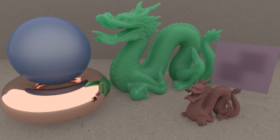
Here are a couple of example materials. Hopefully this is the last programmer art, rendered image I show in the blog until I get to volumetrics :P
From left to right we have:
- Copper torus
- Clearcoat plastic sphere
- Specular transmission with isometric subsurface scattering on the large dragon
- Rough diffuse small dragon
- Thin diffuse transmission on the quad with 2 smaller copper quads behind it.

And for some additional pictures from the Moana Island Scene itself here are two of my favorite elements with lighting of questionable quality. I’ll note that the reason the lighting is bad is because I have almost no tooling for this and iteration is very slow. I definitely need to add some kind of progressive controls in the future.
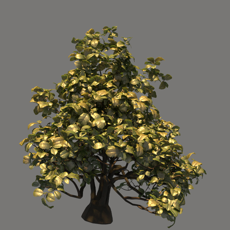
isGardeniaA rendered in my hobby renderer. Clearly the leaves would have subdivision applied to them in Hyperion.
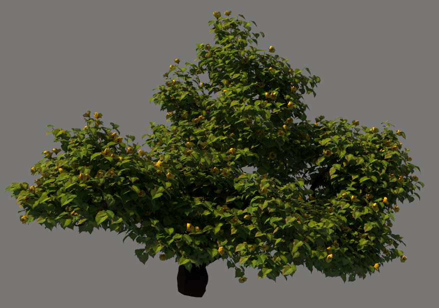
isHibiscus rendered in my hobby renderer
That’s a whole lot of content to take in. I’m sure I left out a handful of details so feel free to ask any questions on twitter. You can also check out my full implementation or my github if you need additional details.
I hope you found this useful! Please leave any feedback here: @schuttejoe!
Updates (10/10/2018):
- Corrected a typo in CalculateExtinction pointed out to me by Syoyo Fujita
- Updated code with much better handling for cases that would lead to NaNs
- Corrected some errors in my pdf calculation. I had often failed to take the Jacobian of the transform applied to the sampled direction into account.
- Added images of isGardeniaA and isHibiscus
References:
- Disney’s Moana Island Scene
- Physically Based Shading at Disney - Burley 2012
- Extending the Disney BRDF to a BSDF with Integrated Subsurface Scattering - Burley 2015
- SIGGRAPH 2012 Course: Practical Physically Based Shading in Film and Game Production
- SIGGRAPH 2015 Course: Physically Based Shading in Theory and Practice
- Disney BRDF Explorer
- Microfacet Models for Refraction through Rough Surfaces
- Memo on the Fresnel Equations
- Understanding the Masking-Shadowing Function in Microfacet-Based BRDFs
- Practical and Controllable Subsurface Scattering for Production Path Tracing
Additional Thanks:
- Morgan McGuire for the cleaned up version of Stanford Graphics Lab’s Chinese Dragon model
- CC0 Textures for the paper texture
- Syoyo Fujita for pointing out a typo in my CalculateExtinction function.