In Part 1 of this post I showed a common method for importance sampling the GGX distribution of normals using the inverse of the CDF of the distribution. While this clearly converged faster than importance sampling a cosine lobe it did still leave a number of fireflys in the image that would be pesky to deal with. Additionally, there is a hidden inefficency that is causing us to potentially waste a number of samples.

In 2014 Eric Heitz and Eugene D’Eon published Importance Sampling Microfacet-Based BSDFs using the Distribution of Visible Normals that describes a method for importance sampling that takes the view direction into account. That solved both of the problems I mention however their method for importance sampling GGX was complicated and not exact. In 2017, Eric Heitz released a technical paper A Simpler and Exact Sampling Routine for the GGX Distribution of Visible Normals that is… exactly what the title says it is. Today, I want to write about these improvements.

---

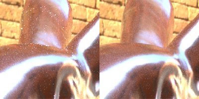
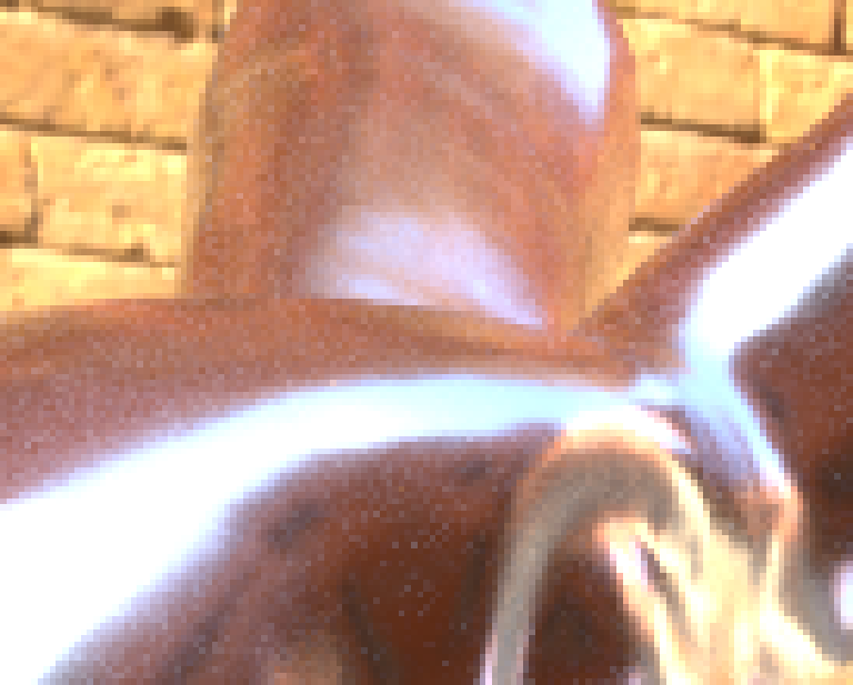
Let’s start by explaining the two flaws with importance sampling only the distribution of normals; fireflys and wasted samples. For those who do not know, a firefly is a term used in rendering to describe a single pixel that is significantly brighter than those in its neighborhood. Let’s zoom in (using nearest-neighbor sampling) on the top of the bunny’s head to see these more clearly.

Earlier I used an image zoomed in on the face but it looked too angry

To understand where the fireflys are coming from we need to take a close look at the pdf used to generate $\wi$ and then think about how that could cause exceptionally bright pixels.

$$\p_i(\wm, \wo) = \frac{\D(\wm)(\wg \cdot \wi)}{4|\wg \cdot \wm|}$$

Now remember that importance sampling works by focusing rays in the directions where they will have a high probabilty of contributing to your image. However, to prevent bias in our results we do have to be sure we can sample the entire range of our function. And, in fact, importance sampling relies on giving those improbable samples a higher weight so that we still arrive at the correct results when that direction does contribute to the image.

Imagine an extremly bright light source shining on a surface from a very low angle when we are looking directly at the surface. If the surface has a low to medium roughness it will be improbable to generate a sample in the direction of that light source but not impossible. In the case where it does we’d expect a low value for $\D(\wm)$, a value close to 1 for $(\wg \cdot \wi)$, and a low value again for $4|\wo \cdot \wm|$. Now our concern here is that if $\p_i(\wm, \wo)$ ends up as a very small number and we then divide that from a large $\L_i(X, \wi)$ we will get a very bright result that will require a significant number of samples in other directions to smooth out. So, given that our weight will be based on the ratio of $\D(\wm)$ to $4|\wo \cdot \wm|$, and given that we can clearly see fireflies in the image from part 1, you can probably guess that there are cases where $\D(\wm)$ is still much smaller than $4|\wo \cdot \wm|$ and we end up dividing by a very small number.

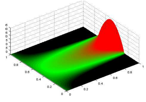
If you don’t like just guessing, Heitz and D’Eon have a diagram in their paper showing the weights we get with values $\xi_0$ and $\xi1$ for a low glancing angle.

For low glancing angles we see a sizable amount of our sample space results in large weights that could cause fireflies

The next problem, wasted samples, is a bit easier to see. Imagine a view vector at a very low glancing angle to a surface with a very high roughness. Because of that high roughness the importance sampling function will generate microfacet normals in a variety of directions across the hemisphere. Now, in all cases where $\wo \cdot \wm \le 0$ we have to discard the entire sample and all of the work that was done by the path tracer for that ray up to that point is now wasted. For a very low glancing angle that can be nearly half of the samples. That’s not good at all!

---

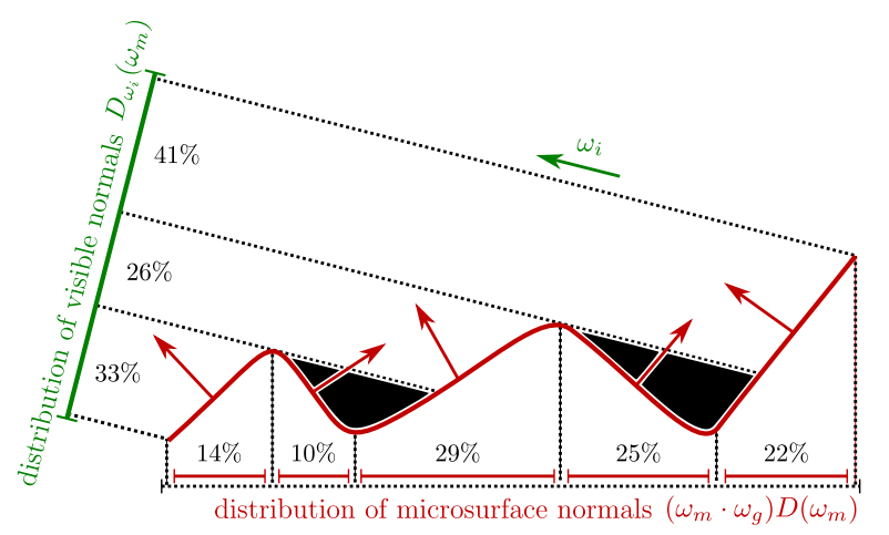
Now that we understand the flaws of importance sampling $\D$($\wm$) let’s look to Heitz and D’Eon and see how they solved these problems. In the 2014 paper Understanding the Masking-Shadowing Function in Microfacet-Based BRDFs Heitz shows the statistical distribution of visible normals. This can be thought of as a function that describes the probabily that a microfacet normal on a surface is visible to the direction $\wo$. This function is defined as:

$$\D_{\wo}(\wm) = \frac{\G_1(\wo, \wm) ~ |\wo \cdot \wm| ~ \D(\wm)}{|\wo \cdot \wg|}$$

In part 1 I reference the Masking-Shadowing function $\G_2(\wi,\wo,\wm)$ but never really explained what it was. Now that we have this new, related, term $\G_1(\wo, \wm)$ show up let’s spend some time on that. $\G_1(\wo, \wm)$ is the statistical masking function that gives the fraction of microfacets that are visible along outgoing direction $\wo$. This definition is local to the surface we are looking at and does not account for any other microgeometry that might later occlude energy as it goes to or reflects from the microfacet. $\G_2(\wi,\wo,\wm)$ on the other hand, should be thought of as the fraction of microfacets that are visible along the outgoing direction $\wo$ AND both the directions $\wo$ and $\wi$ are not occluded by other microgeometry as they go to and leave the microfacet. It’s important to note then that $\G_1(\wo, \wm) \ge \G_2(\wi,\wo,\wm)$. Here is a diagram from [Heitz14] to help visualize.

$\D_{\wo}(\wm)$ only accounts for normals that are visible along $\wo$. Note the change in variables here; they use $\wi$ where I use $\wo$

If we had a way to importance sample $\D_{\wo}(\wm)$ it should be easy to see that the problem of wasted samples will go away since $\wo \cdot \wm$ would always be $\gt 0$. Let’s take a look at what it would do for our firefly problem. If $\D_{\wo}(\wm)$ is the pdf used to sample $\wm$ and we still reflect our view direction over $\wm$ then we have this as our reflectance:

$$\frac{\f(\wi,\wo)| \wg \cdot \wi |}{\p_{\D_{\wm}}(\wm, \wo)} = \frac{\frac{\F(\wi,\wm) ~ \G_2(\wi,\wo,\wm) ~ \D(\wm)| \wg \cdot \wi |}{4 ~ |\wi\cdot\wg| ~ |\wo\cdot\wg|}}{\frac{\G_1(\wo, \wm) ~ |\wo \cdot \wm| ~ \D(\wm)}{|\wo \cdot \wg| ~ 4|\wo \cdot \wm|}} = \boxed{\frac{\F(\wi,\wm) ~ \G_2(\wi,\wo,\wm)}{\G_1(\wo, \wm)}}$$

Well that cleaned up pretty nicely. The best part is since we saw earlier that $\G_1(\wo, \wm) \ge \G_2(\wi,\wo,\wm)$ and we know $\F(\wi,\wm)$ is between 0 and 1 that the weight will be between 0 and 1. No more fireflies!

Ok, great! We just need to actually find a way to importance sample $\D_{\wo}(\wm)$. While the first paper on importance sampling $\D_{\wo}(\wm)$ does propose a solution for GGX with the Smith masking-shadowing function it gets very complicated to understand and relies on a fitted curve. So I’m going to skip ahead to more recent work in the 2017 technical document from Heitz, A Simpler and Exact Sampling Routine for the GGX Distribution of Visible Normals, that I mentioned earlier.

The most confusing part of the document is that Heitz uses the property that with $\a = 1$ the GGX distribution forms a uniform hemisphere. To handle the infinity other cases where $\a \ne 1$ we have to go back to Understanding the Masking-Shadowing Function in Microfacet-Based BRDFs where Heitz shows that we can stretch the distribution of slopes in our masking-shadowing function by changing $\a$ and that this is equivalent to simply changing the slope of the direction we are evaluating.

The statistical masking-shadowing function does not change as it is stretched if we also change the slope of $\omega_x$ accordingly.

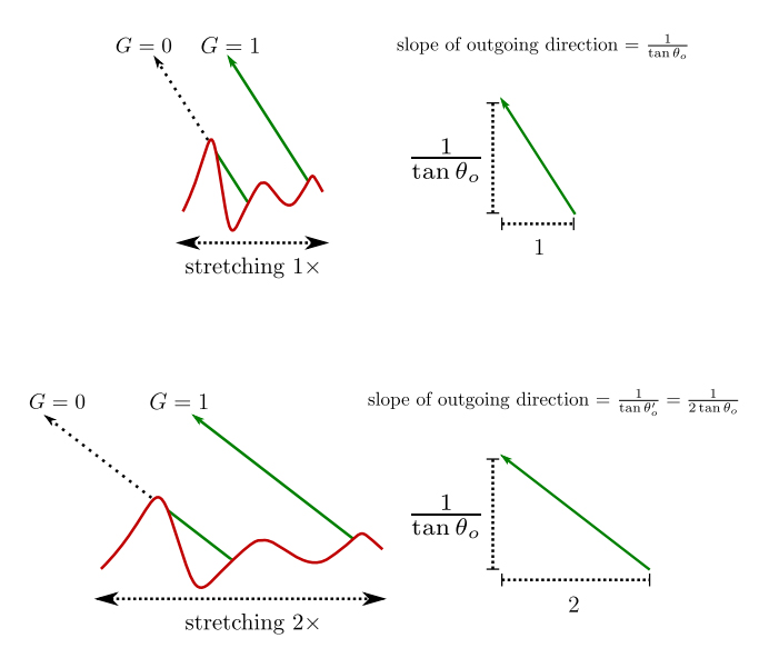
So if we can generate a microfacet normal for $\a=1$ we can stretch it to be usable for any other value of $\a$.

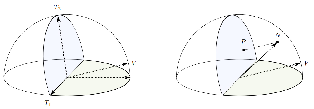
The last thing we need to do is to have a way to uniformly sample only the part of the hemisphere that gives us a microfacet normal $\wm$ where $\wm \cdot \wo \gt 0$. The clever trick that Heitz uses here is to rotate half of the disk upwards so that it is perpendicular to the ray direction $\wo$ then generates samples on the two half disks with probability proportional to its projected area onto direction $\wg$. Then those points are projected onto the hemisphere in the direction of $\wo$ to give us our micofacet normal $\wm$ with $\a=1$. The final step is to apply the stretch to $\wm$ so it is usable for the roughness of the surface we are evaluating.

Heitz and I use different variables again here so let $\textit{V}=\wo$. It should be easy to see how $\wm \cdot \wo \gt 0$ since both directions can be thought of as fitting between those two half disks.

The technical document is quite short and shows the details of the algorithm to generate $\wm$ so I’ll leave that out here and let you check the document for that. Or you can just glean it from the source code below.

---

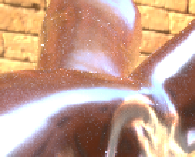
Now let’s compare the results of this new sampling method to the one described in part 1. It might be helpful to zoom in on this one. While the quality difference is much smaller in comparison to the transition from importance sampling the cosine lobe to importance sampling $\D(\wm)$ it is perceptable. Additionally, this new method runs just a little bit faster.

The same scene from part 1. On the left we importance sample $\D(\wm)$ and on the right we importance sample $\D_{\wo}(\wm)$. Both cases still use 512 rays per pixel

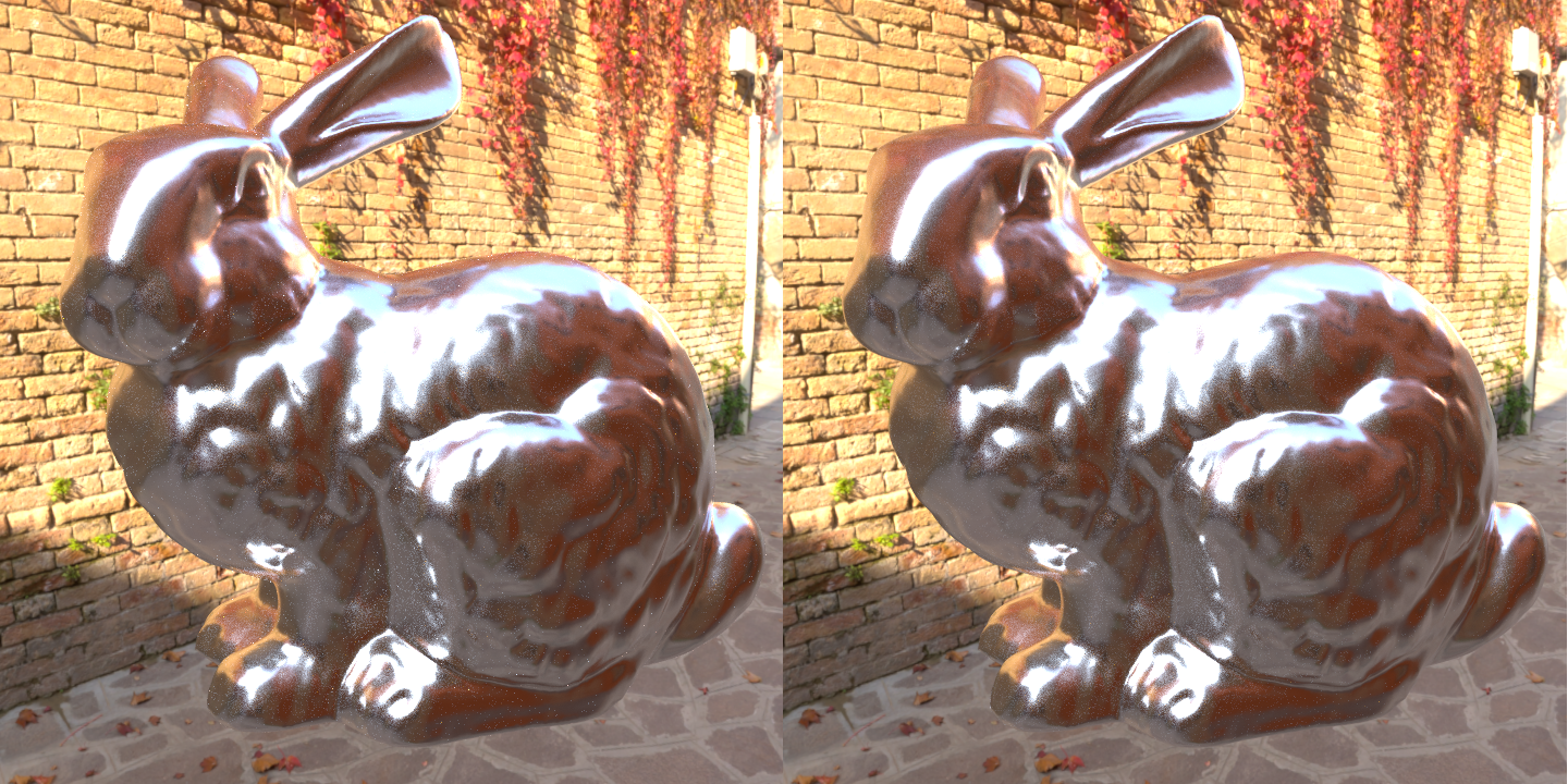
To zoom back in on the bunny’s head we can see that the noise from fireflies is significantly reduced.

Much better! And did I mention this was even a little bit faster?

And finally, here is the source code using this new method to calculate $\wi$ and the reflectance from our surface.

//====================================================================
float SmithGGXMasking(float3 wi, float3 wo, float a2)
{
    float dotNL = BsdfNDot(wi);
    float dotNV = BsdfNDot(wo);
    float denomC = Sqrtf(a2 + (1.0f - a2) * dotNV * dotNV) + dotNV;

    return 2.0f * dotNV / denomC;
}

//====================================================================
float SmithGGXMaskingShadowing(float3 wi, float3 wo, float a2)
{
    float dotNL = BsdfNDot(wi);
    float dotNV = BsdfNDot(wo);

    float denomA = dotNV * Sqrtf(a2 + (1.0f - a2) * dotNL * dotNL);
    float denomB = dotNL * Sqrtf(a2 + (1.0f - a2) * dotNV * dotNV);

    return 2.0f * dotNL * dotNV / (denomA + denomB);
}

//====================================================================
// https://hal.archives-ouvertes.fr/hal-01509746/document
float3 GgxVndf(float3 wo, float roughness, float u1, float u2)
{
    // -- Stretch the view vector so we are sampling as though
    // -- roughness==1
    float3 v = Normalize(float3(wo.x * roughness,
                                wo.y,
                                wo.z * roughness));

    // -- Build an orthonormal basis with v, t1, and t2
    float3 t1 = (v.y < 0.999f) ? Normalize(Cross(v, YAxis_)) : XAxis_;
    float3 t2 = Cross(t1, v);

    // -- Choose a point on a disk with each half of the disk weighted
    // -- proportionally to its projection onto direction v
    float a = 1.0f / (1.0f + v.y);
    float r = Sqrtf(u1);
    float phi = (u2 < a) ? (u2 / a) * Pi_ 
                         : Pi_ + (u2 - a) / (1.0f - a) * Pi_;
    float p1 = r * Cosf(phi);
    float p2 = r * Sinf(phi) * ((u2 < a) ? 1.0f : v.y);

    // -- Calculate the normal in this stretched tangent space
    float3 n = p1 * t1 + p2 * t2
             + Sqrtf(Max<float>(0.0f, 1.0f - p1 * p1 - p2 * p2)) * v;

    // -- unstretch and normalize the normal
    return Normalize(float3(roughness * n.x,
                            Max<float>(0.0f, n.y),
                            roughness * n.z));
}

//====================================================================
void ImportanceSampleGgxVdn(Random::MersenneTwister* twister,
                            float3 wg, float3 wo, Material* material,
                            float3& wi, float3& reflectance)
{
    float3 specularColor = material->specularColor;
    float a = material->roughness;
    float a2 = a * a;

    float r0 = Random::MersenneTwisterFloat(twister);
    float r1 = Random::MersenneTwisterFloat(twister);
    float3 wm = GgxVndf(wo, material->roughness, r0, r1);

    wi = Reflect(wm, wo);

    if(BsdfNDot(wi) > 0.0f) {

        float3 F = SchlickFresnel(specularColor, Dot(wi, wm));
        float G1 = SmithGGXMasking(wi, wo, a2);
        float G2 = SmithGGXMaskingShadowing(wi, wo, a2);

        reflectance = F * (G2 / G1);
        
    }
    else {
        reflectance = float3::Zero_;
    }
}

Thanks again for reading!

Edit 3/12/18: I found an error in the Smith masking and shadowing functions and corrected them.

Edit 3/31/19: Martin Lambers kindly pointed out a shadowed variable in GgxVndf that led to a bug in unstretch.

---

References:

• Understanding the Masking-Shadowing Function in Microfacet-Based BRDFs
• Importance Sampling Microfacet-Based BSDFs using the Distribution of Visible Normals
• A Simpler and Exact Sampling Routine for the GGX Distribution of Visible Normals

Additional thanks to:

• HDRI Haven for the free IBL
• My friends who helped review this.

---

While I had an absolute blast writing this series and I definitely want to write more in the future I’m waiting to gague reactions before I decide how much sense it makes to put effort into the appearance of the site. Until I decide to flesh things out more you can leave comments at:

@schuttejoe