Vertex Connection and Merging
May 29, 2018
$\newcommand{\w}{\textit{w}}$ $\newcommand{\x}{\overline{x}}$ $\newcommand{\B}{\textit{B}}$ $\newcommand{\pf}{\overrightarrow{p}}$ $\newcommand{\pr}{\overleftarrow{p}}$ $\newcommand{\gr}{\overleftarrow{g}}$
If you’re interested in path tracing you’ve probably also at least heard of both bidirectional path tracing (BPT) and photon mapping (PM). Both algorithms were introduced in the 1990s and gave us powerful new tools for solving problems in areas where unidirectional path tracing was weak. However, despite the advancements they offered, neither algorithm saw wide adaptation in film due to some weaknesses of their own. In 2012 [Georgiev et al] introduced an algorithm that combined both of these techniques in a mathematiclaly consistent framework that allowed us to combine both of their strengths into one integrator. That algorithm was called Vertex Connection and Merging (VCM) and is what I’ll be writing about today.
Before I dive straight into an explanation of the VCM algorithm I want to quickly talk about BPT and PM to make sure we’re all clear on how they work and what strengths and weaknesses they have. Before we even get to that I want to also quickly described Multiple Importance Sampling (MIS) since it is at the heart of the BPT and VCM algorithms.
Multiple Importance Sampling
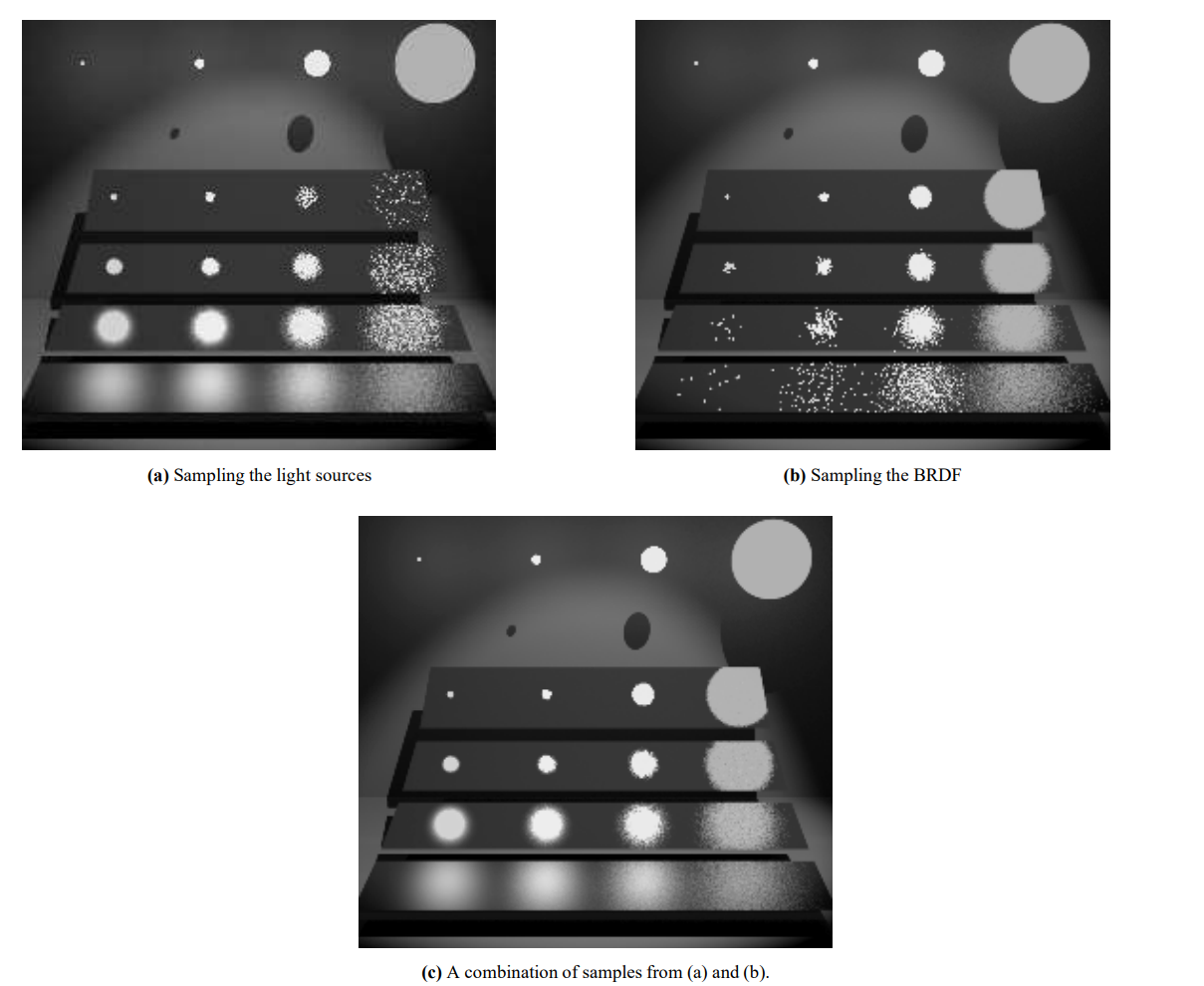
MIS is very useful algorithm when your scene has surfaces that would converge quickly using different importance sampling functions. The algorithm works by choosing samples from more than one function and then weighing each sample in a way that takes the pdf of the other functions being sampled into account. It uses the estimator:
$$I = \sum_{i=1}^n \frac{1}{n_i} \sum_{j=1}^{n_i} w_i(\textit{X}_{\textit{i}, \textit{j}})\frac{f(\textit{X}_{\textit{i}, \textit{j}})}{p_i(\textit{X}_{\textit{i}, \textit{j}})}$$
where n is the number of functions we are importance sampling, $n_i$ is the number of samples we are taking from the $i$th function, and $w_s(\textit{x})$ being a weight function that is usually either the power heuristic:
$$w_s(\textit{x}) = \frac{(n_s * p_s(\textit{x}))^{\textit{B}}}{\sum_{t=1}^{n_t}(n_t * p_t(\textit{x}))^{\textit{B}}}$$
or the balance heuristic which is the above with $\textit{B}=1$.
The benefits here are twofold. The first is that by sampling more than one function we are able to use a sort of aggregate function that more closely fits the integral we are trying to solve. The second is that since each sample weight takes the pdf of every sample function into account we prevent, or at least reduce, the intensity of fireflies as long as at least one of our sampling functions would have a high probably of sampling in the direction of the strong energy source.
The traditional example is a scene with a very rough diffuse surface, a very smooth specular surface, and an area light source. The rough surface will quickly converge when the ray bouce direction is determined via Next Event Estimation (NEE), which is a fancy term for choosing a ray direction that points at a light source. My previous blog post on solid angle sampling of area lights is an example of an efficient way to do this. The smooth surface will converge much more quickly via sampling the BSDF. My first two blog posts cover doing this efficiently for GGX.
Indeed, most places that describe MIS do so in the context of mixing NEE and BSDF sampling but it was actually introduced in Veach and Guibas 1995 for use with bidirectional path tracing.
Bidirectional Path Tracing
What is is: Bidirectional path tracing was independently developed by Lafortune and Williams 1993 and Veach and Guibas 1994. Their idea was that, unlike unidirectional path tracing which only traces paths that originate at the camera, we could trace paths that originate at both the camera and the scene’s light sources then connect those paths together.
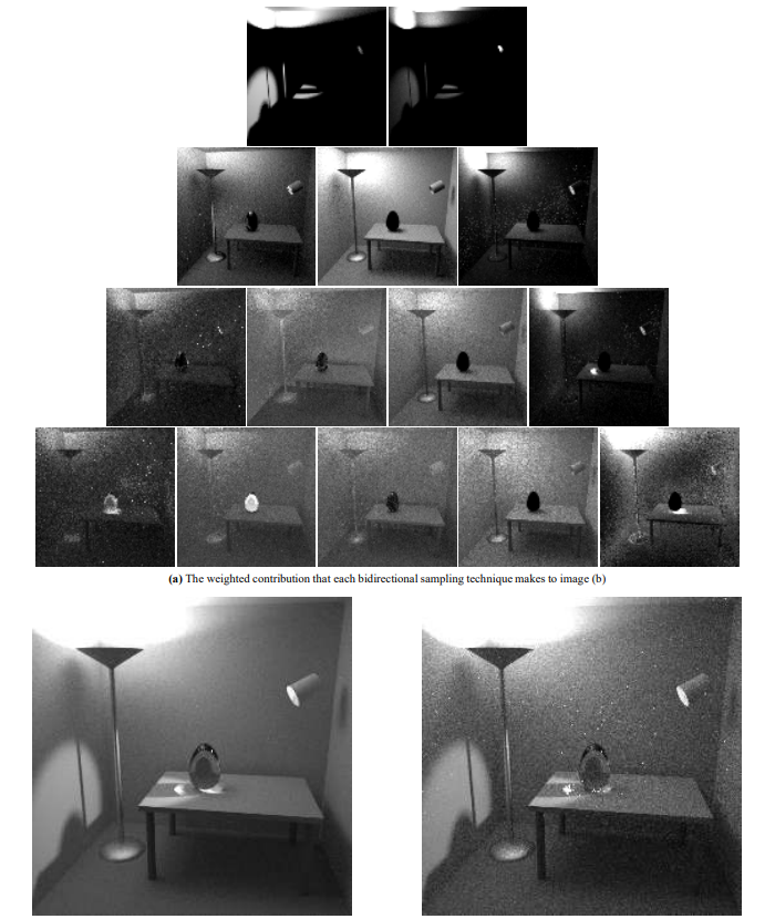
What is it good at: The benefit of BPT is that it works much better for scenes where the light source is “hard to get to” either because it is small or because it requires an unlikely path for it to contribute to the image. Any strong indirect lighting, like in the scene below where most of the scene’s illumination is coming from the light bouncing off of the ceiling, is a great example. Additionally, once we have a full path that connects the camera to a light source we can reduce variance even further by using MIS to weigh each possible way the path could have been constructed: from the camera to the light, from the light to the camera, and each possible pair of connection vertices along the way.
What is it bad at: When using BPT we need to store all of the light paths we traced until a camera path connects to them and this increases the memory footprint of the algorithm as well as its complexity. Additionally, and perhaps worse, without much additional care the coherence of the rays being traced drops considerably given the large variety of origins and sampling techniques being used so that the efficiency of caching and ray batching is decreased.
Photon Mapping
What is it: Photon mapping was introduced by Henrick Wann Jensen in 1996 and is a fairly similar idea to BPT. Under the PM algorithm photons are traced through the scene from each light source and their hitpoints and radiance are stored in a spatial data structure. Then a second pass, called the final gather pass, is done where rays are cast from the camera into the scene and at each hit point all nearby photons are collected and their density is used to estimate the irradiance at that point.
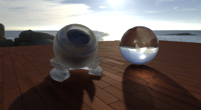
What is it good at: Path reuse! One very powerful aspect of this algorithm is that because each photon cast from a light that finds its way through a complicated transport path (for example, going through a glass sphere) can be used by any number of camera rays duing the final gather. This means that the cost of the work done for that photon was amortized over a potentially large number of camera rays. This makes the algorithm particularly good at handling caustics where light moves through a complicated path and is focused into one area.
What is it bad at: Because the final gather step is based on density estimation the algorithm requires a very large number of photons to achieve smooth results on diffuse surfaces. Large numbers of photons also means a very large memory footprint. This is usually solved via a biased algorithm called Irradiance Caching that only calculates irradiance at some points in the scene and results are interpolated between those points. However, I don’t believe that can be relied on for film where a series of images must have temporal stability to be useful. Additionally, the radius of the final gather introduces a bias (via a blur effect) however that was solved with Progressive Photon Mapping (PPM) which does multiple iterations of the photon mapping algorithm while reducing the radius each iteration and then averaging the results. Finally, it’s error convergence rate has been shown to be relatively slow.
Vertex Connection and Merging
This finally brings us to the VCM algorithm. Once you’re familar with all of the above the idea behind how VCM works becomes fairly simple. What if we traced paths from each light source and stored their hitpoints in a spatial data structure and then when we trace paths from the camera we search the spatial data structure at each hitpoint and connect the paths like in BPT rather than doing a density estimation like PM? While that sounds quite simple the main contribution of the VCM paper was reformulating the search and connection step, called Vertex Merging, into something that works with MIS. In fact, there’s a lot of devil in the details with this algorithm. So much so that the authors also released a technical report and source code explaining how to implement the VCM algorithm. Even with all that they provided it might still be difficult to parse through the algorithm so I’m going to break down some of the details here.
Since I led with a very simplistic description of the algorithm let’s look at a more robust description of what the steps are going to be. Much like PPM, each iteration of the algorithm is split into two passes: the first pass being where we cast light paths from all light sources in the scene and store information about their hit points into a spatial data structure and the second pass being where we cast camera paths camera and perform various types of connections and merging. Here the algorithm diverges from PM and starts to look more like BPT with MIS because it will consider each possible order in which a path could be constructed, as described earlier.
In a complete VCM implementation we will handle each of the follow ways for a path to contribute to the final image:
- Light paths that intersect the camera
- Camera paths that intersect a light source
- Light paths that are connected directly to the camera via NEE
- Camera paths that are connected directly to a light source via NEE
- Camera paths that are connected to a light vertex
- Camera paths that are merged with a stored light vertex
Any time one of these paths contributes to the image we’ll need to calculate the MIS weight for that path taking each possible pdf into account. Like I described in the BPT section, the pdfs we’re calculating at this point are to consider each vertex as having originated at the light, having originated at the camera, or being a merger of a light and a camera vertex. As you can imagine the equations at this point start to get pretty verbose. Here’s the path weight equation in it’s complete form:
$$\w_{v,s,t}(\x) = \frac{n_v^\B p_{v,s,t}^\B(\x)}{n_{VC}^\B \sum_{s’>= 0, t’>= 0} p_{VC,s’,t’}^\B(\x) + n_{VM}^\B \sum_{s’>= 2, t’>= 2} p_{VM,s’,t’}^\B(\x)}$$
That’s a lot to take in and it also sounds like there would be a lot of calculations to make every time a path contibutes to the image. Just touching the memory for each path vertex would be a cache efficency nightmare. Fortunately, in Veach’s dissertation he shows how some terms can be canceled out and Georgiev shows in the technical report a recursive formulation that allows us to compute these weights by tracking only 3 values as we evaluate a path. With those 3 terms, which they call dVCM, dVM, and dVC, calculating the path weight for any of the above 6 cases becomes a fairly quick procedure.
Let’s figure out what those 3 terms we’ll be tracking with each path are: dVCM, dVC, and dVM. To start we’re going to massively simplify the notation for the path weight calculation by reordering the terms in the denominator to group them based on whether they belong to a light or an eye subpath. We also assume we’re using the MIS balance heuristic so $\textit{B}=1$:
$$ \boxed{\w_{v, s, t} = \frac{1}{\w_{v,s}^{light} + 1 + \w_{v,s}^{camera}}}$$
That’s a bit easier on the eyes but we still need to know how to calculate $\w_{v,s}^{light}$ and $\w_{v,s}^{camera}$. The calculations for these are done differently depending on whether the path you are calculating the MIS weight for was completed via vertex connection or vertex merging.
For Vertex Connection we plug $v=vc$ into the weight calculation from earlier and we get:
$$\w_{vc,s}^{light} = \sum_{j=0}^{s-1} \frac{p_{vc,j}}{p_{vc,s}} + \frac{n_{vm}}{n_{vc}} \sum_{j=2}^s \frac{p_{vm,j}}{p_{vc,s}}$$
$$\w_{vc,s}^{camera} = \sum_{j=s+1}^{k+1} \frac{p_{vc,j}}{p_{vc,s}} + \frac{n_{vm}}{n_{vc}} \sum_{j=2}^s \frac{p_{vm,j}}{p_{vc,s}}$$
In both cases we are calculating the weight for the connection happening at vertex $v_s$. For the light sub-path weight we iterate over each vertex on the light sub-path and calculate the ratio of the pdf of the connection happening at $v_s$ to the pdf of the connection at $v_j$. Then we iterate over each vertex on the light sub-path where a merge could occur and sum the ratio of the pdf of a merge happening there to the pdf of the merge happening at $v_s$. For the camera sub-path we perform the same calculation but for the vertices on the camera sub-path. There’s a lot of individual parts here but when it’s all combined together it’s still just the balance heuristic.
If we now look at this with a recursive formulation we can see how each sub-path weight would be modified each time a new vertex is added to that sub-path. For the first vertex on a VC sub-path we’ll get the weight:
$$\boxed{\w_{VC,0} = \frac{\pr_0}{\pf_0}}$$
and each vertex added to the sub-path after that will have the weight
$$\boxed{\w_{VC,i} = \pr_i (n_{VCM} + \frac{1}{\pf_i} + \frac{1}{\pf_i} * \w_{VC,i-1})}$$
Oh boy! More new notation! $n_{VCM} = \frac{n_{VM}}{b_{VC}} \pi r^2$ is the combination of several constants in the path weight into a single term. So, what are those pdf terms and what do the arrows above them indicate? If we have a path $\x_0 \x_1 \x_2 … \x_k$ that advanced from $\x_0$ outwards then $\pf_i$, the forward pdf, is the area pdf for each vertex to connect to its adjacent vertices. With the same path, the reverse pdf $\pr_i$ is the area pdf at each vertex of the path having originated at $\x_k$.
For Vertex Merging we plug $v=vm$ into the weight calculation from earlier and we get the very similar looking:
$$\w_{vm,s}^{light} = \frac{n_{vc}}{n_{vm}} \sum_{j=0}^{s-1} \frac{p_{vc,j}}{p_{vm,s}} + \sum_{j=2}^{s-1} \frac{p_{vm,j}}{p_{vm,s}}$$
$$\w_{vm,s}^{camera} = \frac{n_{vc}}{n_{vm}} \sum_{j=s}^{k+1} \frac{p_{vc,j}}{p_{vm,s}} + \sum_{j=s+1}^{k} \frac{p_{vm,j}}{p_{vm,s}}$$
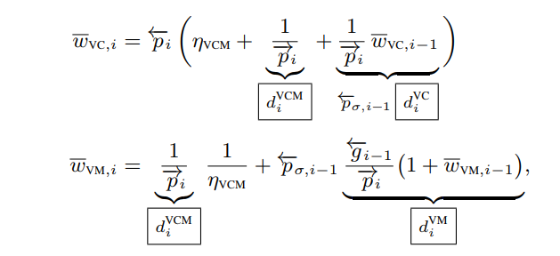
with the recursive formulations being:
$$\boxed{\w_{VM, 1} = \frac{1}{\pf_1} (\frac{1}{n_{VCM}} + \pr \frac{1}{n_{VCM}\pf})}$$
$$\boxed{\w_{VM, i} = \frac{1}{\pf} (\frac{1}{n_{VCM}} + \pr_{i-1} + \pr_{i-1}\w_{VM,i-1})}$$
Calculating dVCM, dVC, dVM:
We’re so close! These recursive formulations look fairly simple and it might seem like we’d only need to track these as we walk the path. Unfortunately, while we’re walking a path we’ll know the direction we leave each vertex in but we won’t know the full area pdf until we also know the distance to the next vertex. This is where Georgiev used the three partial terms dVCM, dVC, and dVM. These are calculated as:
$$ \boxed{d_i^{VCM} = \frac{1}{\pf_i}}$$
$$ \boxed{d_i^{VC} = \frac{1}{\overleftarrow{p}_{\sigma, i-1}} \frac{1}{\pr_i} w_{VC, i-1}}$$
$$ \boxed{d_i^{VM} = \frac{\gr_{i-1}}{\pf_i} (1 + w_{VM, i-1})}$$
where $\overleftarrow{p}_{\sigma, i-1}$ is the solid angle reverse pdf at the previous vertex and $\gr_{i-1}$ is the area measure that converts from a solid angle pdf to area pdf. With these we can quickly construct $\w_{light}$ and $\w_{camera}$ sub-path weights based on whether we’re evaluating a VC or VM connection.
Ok, deep breath everyone. We’ve made it through the math-y part of this post. Let’s discuss the implementation a bit.
Implementation
If you want to skip the explanation and jump straight into the code you can see my implementation or the implementation in SmallVCM. I’m not going to be able to cover all of the details here because there’s so much to cover but I hope to at least help clarify the implementation further.
For each iteration we start by choosing a search radius. In SmallVCM they used this with $a \in [0, 1)$:
$$r(i) = \frac{r_{initial}}{i^{0.5 * (1 - a)}}$$
but any function that goes to 0 at infinity will work. With radius vmSearchRadius the next step is going to be to decide exactly how many paths of each type we want to use per iteration. For each pixel we choose to perform $n_{vc} =$ vcCount vertex connections and then there will be a potential of $n_{vm} =$ vmCount light paths with which we can merge. For SmallVCM they use vmCount = width * height light paths and then they perform vcCount = 1 vertex connection per pixel. With those values we can calculate some constants we’ll need later.
float vmSearchRadiusSqr = vmSearchRadius * vmSearchRadius;
float vmNormalization   = 1.0f / (Math::Pi_ * vmSearchRadiusSqr * vmCount);
float vmWeight          = Math::Pi_ * vmSearchRadiusSqr * vmCount / vcCount;
float vcWeight          = vcCount / (Math::Pi_ * vmSearchRadiusSqr * vmCount);
The next step will be to trace all of the light paths. This will include choosing the starting path vertex on a scene light source, tracing it into the scene to find the next path vertex, calculating the dVCM, dVC, dVM terms, connecting each vertex to the camera, and finally, determining the exit direction based on the BSDF. The pseudocode for these steps looks like:
for(uint i = 0; i < vmCount; ++i) {
    // -- Generate light vertex y_0 from a light source

    while(path length + 2 is less than our max path length) {
        // -- Trace the ray from our most recent path vertex y_j into the scene to find vertex y_j+1
        // -- Update the 3 recursive terms dVCM, dVC, and dVM to account for the area measure of y_j+1 from y_j
        // -- Store the vertex y_j+1 in our spatial data structure
        // -- Connect y_j+1 to the camera
        // -- Sample the bsdf to determine the exit direction for point y_j+1
    }
}
You’ll note that I’m leaving out any handling of the case where the light path intersects the camera directly since I’m still using a pinhole camera that is impossible to hit.
There are a few details here that I will come back to later but for now I want to keep discussing the high level details of the algorithm. Since we’re done creating all of our light paths we’ll usually need to run some setup code for our spatial data structure. I’ll skip the details here and point you at the hash grid implementation from SmallVCM. Once that is done we’re ready to begin the second and final part of the algorithm, tracing the camera paths.
for(uint y = 0; y < height; ++y) {
    for(uint x = 0; x < width; ++x) {
        // -- Generate camera vertex z_0 for point x,y on the camera

        while(path length is less than our max path length) {
            // -- Trace the ray from our most recent path vertex z_j into the scene to find vertex z_j+1
                // -- If the ray leaves the scene we connect it directly to our IBL
            // -- Update the 3 recursive terms dVCM, dVC, and dVM account for the area measure of z_j+1 from z_j
            if path length + 1 is less than our max path length
                // -- Connect vertex z_j+1 to a light source
            // -- Connect vertex z_j+1 to each light vertex from the corresponding light path
            // -- Merge vertex z_j+1 with each light vertex within radius vmSearchRadius
            // -- Sample the bsdf to determine the exit direction for point z_j+1
        }
    }
}
There’s more going on here but much of it is very similar to work that was done during the first pass. I think there are only a few more areas we should talk about before you’ll be ready to write your own VCM integrator. Or at least so you’ll be less confused as you read the source material :P
Generating light and camera vertices
To generate a light vertex we need to first choose a light source in our scene. The probablity of having chosen that light is pdf lightSampleWeight. Then we generate a vertex on that light source and calculate the solid angle pdf for that emission (which includes both the pdf of choosing the vertex position and the pdf of having chosen that sample direction) and we calculate the area pdf of an incoming ray hitting this particular sample. Special care must be taken for an infinite light source like an IBL which is described near the end of the technical report. You can see my implementation for an IBL here. We can then compute our three initial path terms:
sample.emissionPdfW  *= lightSampleWeight;
sample.directionPdfA *= lightSampleWeight;
state.dVCM            = sample.directionPdfA / sample.emissionPdfW;
state.dVC             = sample.cosThetaLight / sample.emissionPdfW;
state.dVM             = sample.cosThetaLight / sample.emissionPdfW * vcWeight;
To generate a camera vertex is a bit simpler. When we set up our camera we calculate the distance the image plane would have to be from the camera such that the area pdf of each pixel is 1.
camera.virtualImagePlaneDistance = imageWidthf / (2.0f * Math::Tanf(horizontalFov));
We then need to calculate the inverse of the solid angle measure to give us the reverse solid angle pdf of the ray leaving the camera. We use that to initialize our three path terms:
float cosThetaCamera = Dot(camera->forward, cameraRay.direction);
float imagePointToCameraDistance = camera->virtualImagePlaneDistance / cosThetaCamera;
float invSolidAngleMeasure = imagePointToCameraDistance * imagePointToCameraDistance / cosThetaCamera;
float revCameraPdfW = (1.0f / invSolidAngleMeasure);

state.dVCM = lightPathCount * revCameraPdfW;
state.dVC  = 0;
state.dVM  = 0;
Updating the 3 recursive terms dVCM, dVC, and dVM
As we process each vertex we will only be able to do a partial update of dVCM, dVC, and dVM since we’ll only have the solid angle pdf and won’t know the area pdf until we cast a ray into the scene and determine the next vertex position and normal. Once we have found the next vertex we can do the second half of the partial update of the 3 terms:
float connectionLengthSqr = LengthSquared(previousPosition - surface.position);
float absDotNL = Math::Absf(Dot(surface.geometricNormal, directionToPreviousVertex));

// -- Update accumulated MIS parameters with info from our new hit position. This combines with work done at the previous
// -- vertex to convert the solid angle pdf to the area pdf of the outermost term.
dVCM *= connectionLengthSqr;
dVCM /= absDotNL;
dVC  /= absDotNL;
dVM  /= absDotNL;
Sampling the BSDF to advance the path
The final iterative step during path evaluation will be to sample the BSDF to determine the direction to trace our next ray in and the corresponding reflectance. Once we’ve chosen our new sample direction we need to calculate the forward solid angle pdf $\overrightarrow{p}_{\sigma, i}$ and the reverse solid angle pdf $\overleftarrow{p}_{\sigma, i}$ which are both used to do a partial calculation of dVCM, dVC, and dVM. For an example you can check out my implementation for a transparent GGX material that samples the visible distribution of normals I described in my second blog post:
dVC = (cosThetaBsdf / sample.forwardPdfW) * (pathState.dVC * sample.reversePdfW + pathState.dVCM + vmWeight);
dVM = (cosThetaBsdf / sample.forwardPdfW) * (pathState.dVM * sample.reversePdfW + pathState.dVCM * vcWeight + 1.0f);
dVCM = 1.0f / sample.forwardPdfW;
Calculating MIS weights to complete a path
Each of the 5 (or 6 if your lens has an area) ways to complete a path that I described earlier requires slightly different work to compute the MIS weight. Rather than make this post even longer than it already is by dumping a bunch of code or math for each of those I’ll just provide links to my implementation of each. Of course, it’s worth noting that I currently only support the 1 scene IBL but adding support for additional area lights should be quite easy.
- Camera paths that intersect a light source
- Light paths that are connected directly to the camera via NEE
- Camera paths that are connected directly to a light source via NEE
- Camera paths that are connected to a light vertex
- Camera paths that are merged with a stored light vertex
Conclusion
While I certainly haven’t shown all of the details involved in implementing VCM I hope I’ve added enough information to make the process clearer to you. Now to show the benefits of using VCM this first image is a scene with some slightly complicated light transport paths and lit only by the scene’s IBL rendered with a unidirectional path tracer:
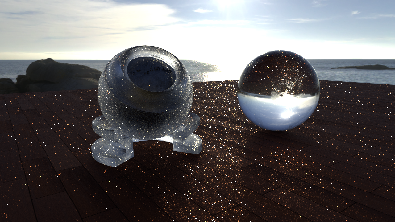
This is very, very far from converging and it’s still quite difficult to even discern what the materials are supposed to look like. Here’s the same scene rendered with VCM given the same amount of time:
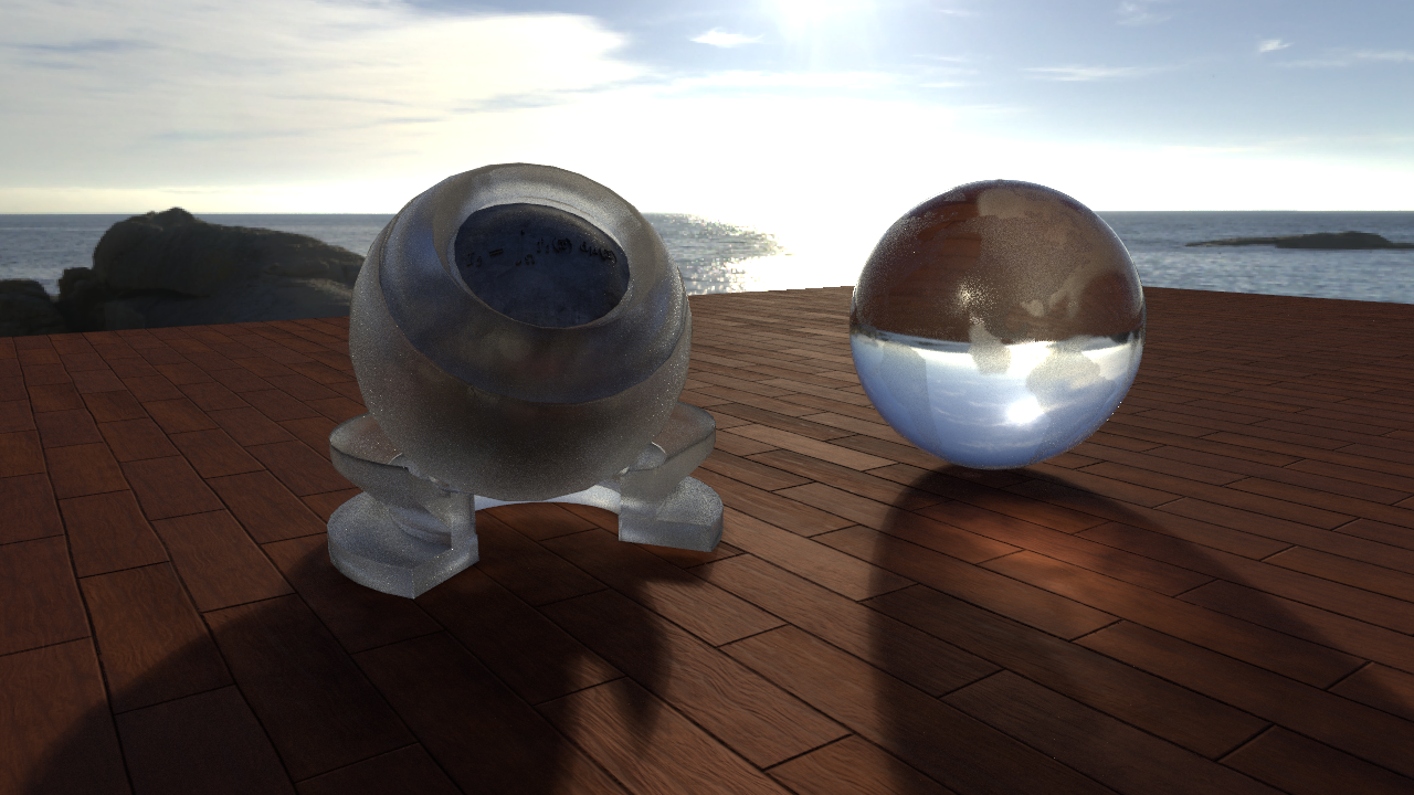
This is still a relatively quick render so if you look closely at the Mori Knob you can see some circular spots that are an artifact of vertex merging. With that said, the results are substantially better than the unidirectional path tracer.
My implementation followed that of SmallVCM where each thread is performing one full iteration of the algorithm which means that the memory overhead for storing light vertices is quite high. I’m also not taking advantage of SIMD lanes and there’s no texture or geometry caching to worry about. At some point in the not-to-distant future I’ll introduce the concepts of ray/shading batches along the lines of what is described in Sorted Deferred Path Tracing in Production Rendering but until I’ve seen how it performs in something that looks like a production environment I will hold off on discussing the pros and cons of the VCM algoritm in more detail.
Thanks again for reading and please leave any feedback here: @schuttejoe!
References:
- Bi-directional Path Tracing - Lafortune and Williams 1993
- Bidirectional Estimators For Light Transport - Veach and Guibas 1994
- Optimally Combining Sampling Techniques for Monte Carlo Rendering - Veach and Guibas 1995
- Light Transport Simulation with Vertex Connection and Merging - Georgiev er al 2012
- Global Illumination Using Photon Maps - Henrick Wann Jensen 1996
- Progressive Photon Mapping - Hachisuka et al 2008
- Implementing VCM - Georgiev 2012
- SmallVCM
- Robust Monte Carlo Methods for Light Transport Simulation - Veach 1997
- Progressive Photon Mapping: A Probabilistic Approach - Zwicker 2011
- Sorted Deferred Path Tracing in Production Rendering - Eisenacher 2013
Additional thanks:
- McGuire Computer Graphics Archive and Yasutoshi Mori for the Mori Knob
- HDRIHaven for the HDRI image used as an IBL